AUTOMATED SOLAR TRACKING SYSTEM FOR PV MODULE
*,1
Ritika Ojha,
2Kranthi Pamarthi Kumar and
1
Oracle
3
National Institute of
ARTICLE INFO ABSTRACT
This paper proposes a novel approach to adjusting the orientation of a Photo
position. The approach implements Kalman Filter algorithm to track maximum power
motor position and piston position. The finite state machine includes five states and is Mealy machine. Using the proposed technique, MPPT can be tracked to an efficiency of 97% within a time as low as 4.5ms. The position of PV array is tracked with an er
carried out in partially shaded and falling irradiance level conditions, and it was found that the proposed method is simple as well as cost effective in comparison to systems using GPS to track the position.
Copyright © 2015 Ritika Ojha et al. This is an open access article distributed under the Creative Commons Attribution License, which permits unrestricted use, distribution, and reproduction in any medium, provided the original work is properly cited.
INTRODUCTION
Renewable sources of energy are more abundant than the traditional fossil fuels and ideally, they are enough to easily supply world's energy needs. The surface of earth receiver around 89PW of total incoming solar
even, it would be sufficient to meet our requirements. The solar radiations received can be transformed into electrical energ using Solar Cells which generate electrical energy by Photo
semi-conductor material when exposed to light. Photovoltaic power generation is achieved using solar panels. setback in using a PV panel is that its output non
temperature, solar insolation, etc. This poses a huge risk while using it. The entire PV array does not receive equal amount radiations at all times. Sometimes, parts of the array are under shading due to clouds,
in occurrence of multiple peaks in the Power versus Voltage characteristics of the array which hinders the proper functioning maximum power point tracker. Considerable power will be lost if local maximum
maximum. Hence it is pertinent to track the optimal operating voltage of the output of a PV array for better efficiency of PV generators. The PV array gives different output at different times of day for differ
sunlight falling on the module, and the angle at which the rays fall on it. panel to optimize the power output of panel. It provides an efficient tech respect to the ground so as to obtain maximum output from the module at all times.
MPPT Tracking using Kalman Filters
PV array consists of collection of numerous solar cells in series or parallel to shows the equivalent circuit model of a solar cell. R
simplify the electrical model.
*Corresponding author: Ritika Ojha,
Oracle Financial Services Software Ltd, Mumbai, India.
ISSN: 0975-833X
Article History:
Received 10th July, 2015
Received in revised form
29th August, 2015
Accepted 15th September, 2015
Published online 31st October,2015
Citation: Ritika Ojha, Kranthi Pamarthi Kumar and Dr. Umesh Chandra Pati
International Journal of Current Research, 7, (10
Key words:
Maximum power-point tracking, Melay type state machine, Kalman filters.
RESEARCH ARTICLE
AUTOMATED SOLAR TRACKING SYSTEM FOR PV MODULE
Kranthi Pamarthi Kumar and
3Dr. Umesh Chandra Pati
Oracle Financial Services Software Ltd, Mumbai
2
University of Cincinnati, Ohio
National Institute of Technology, Rourkela
ABSTRACT
This paper proposes a novel approach to track the solar position and hence, a suitable position for adjusting the orientation of a Photo-voltaic array so as to attain more energy than an array in fixed position. The approach implements Kalman Filter algorithm to track maximum power
motor position and piston position. The finite state machine includes five states and is Mealy machine. Using the proposed technique, MPPT can be tracked to an efficiency of 97% within a time as low as 4.5ms. The position of PV array is tracked with an error of ±2%. Experiments have been carried out in partially shaded and falling irradiance level conditions, and it was found that the proposed method is simple as well as cost effective in comparison to systems using GPS to track the position.
This is an open access article distributed under the Creative Commons Attribution License, which permits unrestricted use, distribution, and reproduction in any medium, provided the original work is properly cited.
Renewable sources of energy are more abundant than the traditional fossil fuels and ideally, they are enough to easily supply world's energy needs. The surface of earth receiver around 89PW of total incoming solar insolation. If we capture less than 0.02% even, it would be sufficient to meet our requirements. The solar radiations received can be transformed into electrical energ using Solar Cells which generate electrical energy by Photo-Voltaic effect i.e. building of Voltage or Direct Electric Current in a
conductor material when exposed to light. Photovoltaic power generation is achieved using solar panels.
setback in using a PV panel is that its output non-linear in nature and it greatly varies with environmental changes like temperature, solar insolation, etc. This poses a huge risk while using it. The entire PV array does not receive equal amount radiations at all times. Sometimes, parts of the array are under shading due to clouds, tree, buildings, towers, dust, etc. This results in occurrence of multiple peaks in the Power versus Voltage characteristics of the array which hinders the proper functioning maximum power point tracker. Considerable power will be lost if local maximum power point is tracked instead of the global maximum. Hence it is pertinent to track the optimal operating voltage of the output of a PV array for better efficiency of PV generators. The PV array gives different output at different times of day for different orientations depending upon the amount of sunlight falling on the module, and the angle at which the rays fall on it. This paper deals with solving these issues by adjusting the panel to optimize the power output of panel. It provides an efficient technique to rotate the panel to an appropriate angle with respect to the ground so as to obtain maximum output from the module at all times.
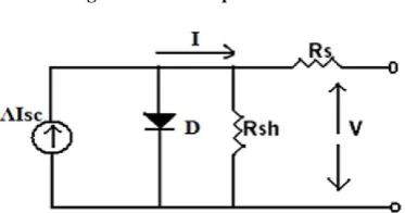
PV array consists of collection of numerous solar cells in series or parallel to get the desired voltage and current. Following figure shows the equivalent circuit model of a solar cell. Rs is very small, Rsh is very large and hence, both can be ignored so as to
cle Financial Services Software Ltd, Mumbai, India.
International Journal of Current Research
Vol. 7, Issue, 10, pp.22018-22025, October, 2015
Ritika Ojha, Kranthi Pamarthi Kumar and Dr. Umesh Chandra Pati, 2015. “Automated solar tracking system for PV module , 7, (10), 22018-22025.
AUTOMATED SOLAR TRACKING SYSTEM FOR PV MODULE
Dr. Umesh Chandra Pati
track the solar position and hence, a suitable position for voltaic array so as to attain more energy than an array in fixed position. The approach implements Kalman Filter algorithm to track maximum power-point (MPPT), motor position and piston position. The finite state machine includes five states and is Mealy machine. Using the proposed technique, MPPT can be tracked to an efficiency of 97% within a time ror of ±2%. Experiments have been carried out in partially shaded and falling irradiance level conditions, and it was found that the proposed method is simple as well as cost effective in comparison to systems using GPS to track the
This is an open access article distributed under the Creative Commons Attribution License, which permits unrestricted use,
Renewable sources of energy are more abundant than the traditional fossil fuels and ideally, they are enough to easily supply the insolation. If we capture less than 0.02% even, it would be sufficient to meet our requirements. The solar radiations received can be transformed into electrical energy by lding of Voltage or Direct Electric Current in a conductor material when exposed to light. Photovoltaic power generation is achieved using solar panels. However, a major y varies with environmental changes like temperature, solar insolation, etc. This poses a huge risk while using it. The entire PV array does not receive equal amount of tree, buildings, towers, dust, etc. This results in occurrence of multiple peaks in the Power versus Voltage characteristics of the array which hinders the proper functioning on power point is tracked instead of the global maximum. Hence it is pertinent to track the optimal operating voltage of the output of a PV array for better efficiency of PV ent orientations depending upon the amount of This paper deals with solving these issues by adjusting the nique to rotate the panel to an appropriate angle with
get the desired voltage and current. Following figure is very large and hence, both can be ignored so as to
OF CURRENT RESEARCH
Fig. 1. Solar cell equivalent circuit
The simplified equation to describe the PV panel is,
Where, Isc and Voc are open circuit current and voltage values at 1kW/m2 and 250C. T is the temperature of array in 0 o
C, q is the elementary charge, λ is irradiance in kW/m2, k is the Boltzmann constant and A is a scalar constant (~0.2464). V and I are the voltage output and current output, respectively, of the PV array.
According to PV curve of PV cell, power increases with a gradual positive slope till an optimal point and then decreases steeply. The voltage output from module is passed into Kalman Filter.
Let Vact be the process, Vactt be the known state. Then,
Vactt+1 = Vactt + M(ΔP/ΔV) + w
Here A = 1; B = M
Let Vref be module output,
Vreft+1 = Vactt+1 + v
Voltage estimate priori at t+1 is,
Vactt+1 = Vact-t + M(ΔP-t/ΔV-t) (1)
The process noise is assumed to be zero initially
Priori estimate of error covariance is,
zt-+1 = zt + Q(2)
Measured voltage is,
Vreft+1 = Vact-t+1 + v(3)
Here C = 1
Equation (1) and (2) form the prediction state.
The Kalman gain is,
Kt+1 = zt-+1(zt-+1 + R)-1(4)
Vactt+1 = Vact-t+1 + Kt+1[Vreft+1 - Vact-t+1](5)
Posteriori error covariance estimate is,
Zt+1 = Zt-+1(1 - Kt+1)(6)
Equations (4), (5) and (6) will form the correction states.
Rotation Mechanism for PV Module
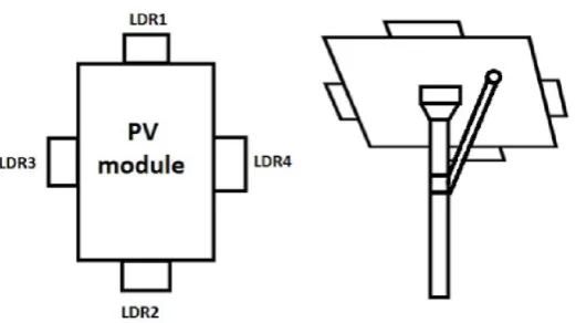
[image:3.595.169.430.280.426.2]The proposed design for mount uses a motor and solenoid powered cylinder to support rotation of the module towards sun. The piston length of cylinder is calculated during the implementation for a rectangular module. The module is supported on the shaft by a motor which is attached to rotate the module in horizontal direction. The contact of module and shaft is made in such a way that the module is hinged in the shaft to facilitate its vertical rotation. A solenoid powered cylinder is mounted in the shaft such that the piston head is attached exactly at a quarter length of the module from hinge center. This helps for vertical movement of module as we do not require entire rotation. A rotation of about 30degrees odd is required as we don’t want the module to be perfectly perpendicular to the incident light. For maximum output power, we use both these steps to position PV module.
Fig. 2. Design of mount (a) Top View (b) Rear View
From the figure we can observe how the shaft is hinged to the module and how the solenoid powered cylinder piston head is attached to the module. The piston will be completely-out during the noon hours and completely-in during the early hours of sunrise and sunset. For technical feasibility, we consider only 4 LDR circuitry in the module. The output of LDR3 and LDR4 is used for horizontal displacement and LDR1 and LDR2 is used for vertical displacement.
Let V1 and V2 be voltages of LDR 1 and LDR2 and V3 and V4 be voltages of LDR3 and LDR4.
Two essential components used for the control of the mount in respect to position are motor and the cylinder. Motor is used to rotate the panel to required position both in clockwise and anti-clockwise direction. Cylinder is used to elevate the panel to the required position by extending or retracting the piston. The directions in both cases are found out based on LDR sensor output and self-regulatory control is to be achieved by using Kalman filter to estimate required rotation.
Motor Algorithm
This is the first phase of movement control. LDR sensor 3 and 4 are used as primary control input to the system. Voltages at hand are V3 and V4. To find necessary rotation, first we need to find out which of the voltages is more. The rotation takes place towards
higher voltage side.
The magnitude of rotation is known from the difference of average of 2 known voltages and their range.
Ideally, the rotation stops when average value is equal to the lower voltage value.
Let Vm1 = V3 - V4
Vm2 = (V3 + V4)/2
When Vm1>0, V3>V4, rotation takes place towards LDR3 an stops when V4 = Vm2
Kalman filter implementation
Let ϴ be the process and ϴt-1 be the known state
Measured variable is the high irradiance position at a particular time during the day.
Let it be ϴref
We have,
ϴt = ϴt-1 + MU
Here A = J and B = M
Rotation estimate priori at ‘t’ is,
ϴ̂t- = ϴ̂t-1 + MU ………. (1)
The process noise is assumed to be 0 initially
Priori estimate of error covariance is,
Zt- = Zt-1 + Q ……….. (2)
Measured rotation is,
ϴref t = ϴ̂t- + MU ……… (3)
Here c = 1
Equation (1) and (2) form prediction state
The Kalman Gain is calculated from formulae,
Kt = zt-cT/(czt-cT + R)
Since c=I in our requirement,
Kt = zt-(zt- + R)-1 ……… (4)
Posteriori rotation estimate is,
ϴ̂t = ϴ̂t- + Kt[ϴref t - ϴ̂t-] ………... (5)
Equation (4), (5) and (6) form correction step
Control Element (MU):
From equation (1) in previous algorithm,
ϴ̂t = ϴ̂t-1 + MU
MU is dimensionless quantity in radians.
Sources in hand are two voltages V3 and V4
From control algorithm, control factor
U = Vm2 - (V3-V4)
The unit of M should be degrees/V
Ideal case: Let V3 has maximum and V4 has minimum measurable voltage on the panel
(Vmax - Vmin)V = 180
1V = 180/(Vmax - Vmin)
Number of degrees/Volt = 1/(Vmax - Vmin)/180
Number of Volts = Vm2 - (V3 or V4)
Total length to be covered = (Number of degrees/Volt)*radius
Total control element is MU = Total length to be covered* Number of Volts/Radius in consideration
Dimensional Analysis: degree*l*V/(V*l)=degrees
Hence control element,
MU = 180/(Vmax - Vmin)
Cylinder algorithm
This is the phase-2 of movement control. LDR sensor 1 and 2 are used as primary control input to the system. Voltages at hand are V1 and V2. To find necessary rotation, first we need to find out which voltage is more. The rotation takes place towards higher
voltage side. The magnitude of translation is known from the difference of average of 2 known voltages and difference of 2 known voltages.
Ideally the translation stops when average value is equal to low voltage.
Let Vt1 = V1 - V2
Vt2 = (V1 + V2)/2
When Vt1>0, V1>V2, translation takes place towards LDR1 an stops when V2 = Vt2
When Vt1<0, V1<V2, translation takes place towards LDR2 and stops when V1 = Vt2
Kalman filter implementation
Let L be the process and Lt-1 be the known state measured variable is the high irradiance position at a particular time during the
day.
Let it be Lref
We have,
Lt = Lt-1 + MU
Here, A = I and B = M
Therefore, translation estimate priori at t is,
Lt = Lt-1 + MU(1)
The process noise is assumed to be zero initially.
Prior estimate of error covariance is,
Zt = Zt-1 + Q(2)
Lref t = Lt + V(3)
Here C = I
Equation (1) and (2) form the prediction state of the control estimates are estimated now. The kalman gain is calculated from the formula,
Kt = zt-cT/(czt-cT + R)
Since c=I in our requirement,
Kt = zt
-(zt -
+ R)-1(4)
Posteriori translation estimate is,
L̂t = L̂t -
+ Kt[Lref t - L̂t
-](5)
Posteriori error covariance estimate is,
zt = zt -
- Ktzt -
zt = zt-(1 - Kt)(6)
Equations (4), (5) and (6) for the correction step for the estimated estimates previously.
Control Element (MU)
From equation (1) in the previous algorithm,
L̂t = L̂t-1 + MU
MU is a dimensional quantity with unity length.
Sources at hand are two voltages V1 and V2 and the radius of the panel in consideration. Assuming cylinder head contacts the
panel at r/2 when r is the radius.
Control factor U = Vt2 – (V1 or V2 )
The unit of U is volts thus V. Unit of M should be L/V
Ideal case: let V1 has maximum and V2 has minimum measurable voltage at panel
(Vmax – Vmin) V =180
1 V= 180/(Vmax – Vmin) degrees
1 V = π/(Vmax – Vmin) radians
Number of radians per volt = π/(Vmax – Vmin) radians
Number of volts = (Vt2 – (V1 or V2)) volts
Total length to be covered = (number of radians per volt) * (radius)
= π/( Vmax – Vmin) * r
Total control element is MU
= (total length to be covered/ radius) * (distance from centre to cylinder head) * (number of volts)
MU= r[Vt2 – (V1 or V2)] / 2(Vmax – Vmin) * π
Therefore M= r / 2(Vmax – Vmin) * π
Where r is the radius of the panel
Finite State Model for System
The system is carried out in 5 states:
Initial State1 State2 State3 State4
Here all the in-built values are taken as input but no output is taken. It forms the base step and keeps ready the data required for computation.
This state carries out only the MPPT process. This state is used when there is no need for movement of motor and piston.
This state carries out all the instructions in MPPT process and motor process. This is used when motor movement is required but not piston movement.
This state carries out all the instructions in MPPT process and piston process. This is used when piston movement is required but not motor movement.
This state carries out all the instructions in MPPT process, motor process and piston process. This is used when both motor and piston movement required.
[image:7.595.39.564.171.241.2]One specific requirement is that MPPT process must run all along the time while motor and piston movement need not run all the time. Initial stage is fed to the system reset. When reset is high, the system stops working and 0 is passed to all outputs.
Fig. 3. Finite State Model for Solar Tracker
Table 4. State Encoding
Name State4 State3 State2 State1 Initial
Initial 0 0 0 0 0
State1 0 0 0 1 1
State2 0 0 1 0 1
State3 0 1 0 0 1
State4 1 0 0 0 1
Simulation Results and Discussion
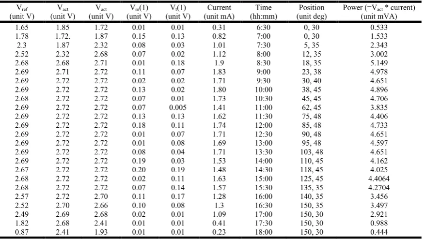
For implementation purpose, a 2.75V (open circuit voltage) and 2 mA (short circuit voltage) solar panel is used. It produces 5.5mW at 250c and 1KW/m2 irradiance. MPP varies from 1.7V to 2.75V depending upon environmental conditions. MPPT algorithm, motor algorithm and piston algorithm are implemented individually on cyclone-II, EP2C20F484C7 as implementation in reconfigurable architecture like FPGA ensured hardware based flexibility. However, the computational complexity of all the three processes combined together and also the pin count is more than the capacity of EP2C20F484C7. So the total system has been simulated using cyclone-IV GX EP4CGXII0DF31C8.
Resource utilization:
Total logic elements- 29,794 (27%) Total register- 21,571
Total pins- 304
Total memory bits- 6,954(<1%)
[image:7.595.156.440.291.423.2]Table 5. Observations under partially shaded condition using algorithm (implementing MPPT)
Vref
(unit V)
Vact
(unit V)
Vact
(unit V)
Vm(1)
(unit V)
Vt(1)
(unit V)
Current (unit mA)
Time (hh:mm)
Position (unit deg)
Power (=Vact * current)
(unit mVA)
1.65 1.85 1.72 0.01 0.01 0.31 6:30 0, 30 0.533
1.78 1.72. 1.87 0.15 0.13 0.82 7:00 0, 30 1.533
2.3 1.87 2.32 0.08 0.03 1.01 7:30 5, 35 2.343
2.52 2.32 2.68 0.07 0.02 1.12 8:00 12, 35 3.002
2.68 2.68 2.71 0.01 0.18 1.9 8:30 18, 35 5.149
2.69 2.71 2.72 0.11 0.07 1.83 9:00 23, 38 4.978
2.69 2.72 2.72 0.02 0.02 1.71 9:30 30, 40 4.651
2.69 2.72 2.72 0.13 0.02 1.80 10:00 38, 45 4.896
2.68 2.72 2.72 0.07 0.01 1.73 10:30 45, 45 4.706
2.69 2.72 2.72 0.07 0.005 1.41 11:00 62, 45 3.835
2.69 2.72 2.72 0.13 0.13 1.62 11:30 75, 48 4.406
2.69 2.72 2.72 0.18 0.11 1.74 12:00 85, 48 4.733
2.69 2.72 2.72 0.01 0.07 1.71 12:30 90, 48 4.651
2.69 2.72 2.72 0.01 0.08 1.69 13:00 95, 48 4.597
2.69 2.72 2.72 0.08 0.04 1.71 13:30 103, 48 4.651
2.69 2.72 2.72 0.19 0.03 1.53 14:00 110, 45 4.162
2.67 2.72 2.72 0.20 0.19 1.48 14:30 118, 45 4.025
2.68 2.72 2.72 0.02 0.11 1.63 15:00 125, 45 4.4064
2.68 2.72 2.72 0.07 0.14 1.57 15:30 135, 35 4.2704
2.57 2.72 2.70 0.11 0.17 1.28 16:00 140, 35 3.456
2.52 2.70 2.66 0.10 0.08 1.3 16:30 150, 35 3.497
2.49 2.69 2.68 0.02 0.01 1.09 17:00 150, 30 2.921
1.82 2.68 2.41 0.01 0.01 0.41 17:30 150, 30 0.988
0.87 2.41 1.93 0.01 0.01 0.23 18:00 150, 30 0.444
Conclusion
By using Kalman Filter algorithm to track MPPT, motor position and positon position, an optimum position for a PV array to operate was found. This is achieved by using maximum power point tracking and adjusting of panels at an orientation which yields maximum power output. MPPT was tracked up to an efficiency of 97% within a time of about 4.5ms. The position of PV array was tracked to an error of ±2% mostly. Further work can be carried out to increase the efficiency of algorithm and improve hardware flexibility.
REFERENCES
Greg Welch and Gary Bishop, 2006. “An Introduction to the Kalman Filter”. University of North Carolina at Chapel Hill, Chapel Hill, NC 27599-3175.
Kalman, R.E. 1960.“A new approach to linear filtering and prediction problems”. Journal of Basic Engineering, Vol. 82. Kang, B.O. and Park, J.H. 2011. “Kalman filter MPPT method for a solar inverter”. Power and Energy Conference at Illinois
(PECI), IEEE.
Kumar, Pamarthi Kranthi and Ojha, Ritika, 2013. “Solar Tracker System for PV Module”. BTech thesis.
Mellit, H., Rezzouk, A., Messai, B. and Medjahed, May, 2011. “FPGA-based real time implementation of MPPT-controller for photovoltaic systems”. Renewable Energy, Volume 36, Issue 5.
Trishan Esram and Patrick L. Chapman, June, 2007. “Comparison of Photovoltaic Array Maximum Power Point Tracking Techniques”. IEEE Transactions on Energy Conversion, Vol. 22, No. 2.
Varun Ramchandani and Kranthi Pamarthi, May, 2013.“Implementation of maximum power point tracking by using Kalman filter for solar PV array on FPGA”.International Journal of Smart Grid and Clean Energy,Vol. 2, no. 2.