doi:10.4236/jilsa.2011.34027 Published Online November 2011 (http://www.SciRP.org/journal/jilsa)
A New Weight Initialization Method Using
Cauchy’s Inequality Based on Sensitivity Analysis
Thangairulappan Kathirvalavakumar1, Subramanian Jeyaseeli Subavathi2
1
Department of Computer Science, V.H.N.S.N. College, Virudhunagar, India; 2Department of Information Technology, Sri Kaliswari College, Sivakasi, India.
Email: [email protected],[email protected] Received June 7th, 2011; revised July 7th, 2011; accepted July 30th, 2011.
ABSTRACT
In this paper, an efficient weight initialization method is proposed using Cauchy’s inequality based on sensitivity analy- sis to improve the convergence speed in single hidden layer feedforward neural networks. The proposed method ensures that the outputs of hidden neurons are in the active region which increases the rate of convergence. Also the weights are learned by minimizing the sum of squared errors and obtained by solving linear system of equations. The proposed method is simulated on various problems. In all the problems the number of epochs and time required for the proposed method is found to be minimum compared with other weight initialization methods.
Keywords: Weight Initialization, Backpropagation, Feedforward Neural Network, Cauchy’s Inequality, Linear System of Equations
1. Introduction
The error backpropagation method has been greatly used for the supervised training of feedforward neural netwo- rks (FNN). But the main drawback of this method is its slow convergence. Many techniques have been proposed to speed up this method, such as second order algorithms [1,2], adaptive step size method [3,4], least squares meth- od [5-7] and appropriate weight initialization method [7-9]. In the following, we discuss some techniques to determine the initial weights of the network.
Shimodaira [10] has proposed a weight initialization method (OIVS) based on geometical considerations to improve the learning performance of the backpropaga-tion algorithm in neural networks. This method is based on the equations representing the characteristics of the information transformation mechanism of a node. Drago and Ridella [8] have proposed a method called SCAWI to improve the performance of the backpropagation algo-rithm. In this method, the authors use the concept of “Paralyzed neuron percentage” (PNP) which describes how many times a neuron is in a saturated state and the magnitude of atleast one output error is high.
Lehtokangas et al.[11] have proposed a method for
weight initialization based on the orthogonal least squares problem. Liu et al. [12] have proposed weight in- itialization of FNN by means of Partial Least Squares.
This method ensures that the output of neurons are in the active region and increases convergence rate. Zhang et al. [13] have proposed a weight initialization method based on estimating the complexity of a function. Then the op-timal network size and topology have been selected and weights are obtained. Nguyan and Widrow (NW) [9] have proposed a weight initialization method by distributing the initial weights of the hidden neurons. So that each hidden node is assigned to a portion of the range of desir- ed function at the start of training.
Fernandez-Redondo and Hernandez-Espinosa [14] pre-sented a paper by comparing six different weight initiali- zation methods with two training algorithms and six da-tabases. The comparison is performed by measuring spe- ed of convergence, generalization and probability of con- vergence. A partial least squares (PLS) algorithm is used in [15] together with the backpropagation algorithm to calculated both the initial weight values and the optimal number of hidden neurons. The PLS structure is viewed as a simplified three layered ANN and its basic funct ion is to reduce the number of input variables.
can be computed analytically with linear least squares. It is a novel method of backpropagating the desired respon- se through the layers of a multilayer perceptron.
Yam et al. [7] have proposed a method to find optimal initial weights based on a linear algebraic method. In each layer least squares method is used to find the wei- ghts. Yam and Chow [18,19] have proposed two methods for weight initialization. In the first method the weights are determined based on Cauchy’s inequality and a linear algebraic method which confirms that the outputs of neurons are in the active region and increases the rate of convergence. In the second method the initial weight vectors are determined based on multidimensional ge-ometry. This method also ensures that the outputs of neu-
rons are in the active region. Castillo et al. [20] have
proposed a method to determine the weights in one layer feedforward neural networks by minimizing either sum of squared errors or the maximum absolute error. Here weights are obtained by solving linear system of equa-tions. Castillo et al. [21] have also proposed another me- thod based on sensitivity of all parameters with respect to its inputs and outputs of each layer. The method is used for neural network learning and also as the initial method to find the weights.
[image:2.595.65.287.561.703.2]In this paper, a new approach to determine the initial weights of single hidden layer feedforward neural net-work is proposed. In the proposed method, the derivative of the activation function is set to a large value [18] to ensure the hidden neuron’s outputs are in the active re-gion. Then Cauchy’s inequality is applied to assign initial weights for the hidden layer and the outputs of hidden layer is calculated. Next linear system of equations de- fined by Castillo et al. [20] are applied to calculate the weight vectors of both the layers. Since this method en- sures hidden neurons outputs are in the active region, the initial weights calculated increases the speed of conver- gence. The efficiency of the proposed algorithm in terms of epochs and time is shown by the simulation result of
Figure 1.Two layer feedforward neural network.
the selected problems namely Iris data set, two spirals problem, modeling a three input nonlinear function, func- tion approximation problem and breast cancer problem. The proposed training method is presented in section 2. Section 3 describes the simulation results of the selected examples.
2. Training of Neural Network
The single hidden layer neural network as in Figure 1 con- sists of I number of inputs xip including bias, J number
of outputs jp, K number of hidden units with outputs
kp, where p refers the patterns considered in training
and T is the target matrix. The input and hidden layer has
one bias neuron with 0p
y z
1
x and z0p 1. and
1
ki
w w2jk
1
w
are weights of hidden layer and output layer respectively.
The net value of hidden layer is obtained by ip ki.
Then the output of the hidden layer is . Here
kp
k
z f O x
kp
O
kp
f x is the sigmoidal activation 1 1
x
e
with
range 0 to 1 used in both hidden and output layer.
2.1.Training Method
In general weights are updated using the mean squared error as cost or error function. The function calculates the error by taking the difference between actual and desired output. Here the hidden layer output z are assumed to be known. The cost function [21] defined for this network is
1
2
Q z Q z Q z
1
1
2 1
1
0
2
1 1 2
2
1 0
I
ki ip k kp
P K
i
J K
p k
jk kp j jp
j k
w x f z
Q z
w z f y
(1)
This cost function is based on the sum of squared er-rors obtained independently by the hidden and output layers. In general, the change of weight depends on the outputs of neurons connected to it. When the outputs of neurons are 0 or 1, the derivative of the activation func-tion is 0. Therefore there will be no weight change at all, even if there is a difference between the value of the tar-get and the actual output. To obtain maximum value for the network weights and also to ensure the outputs of hidden units are in the active region, the weights are ob-tained by using the following equation defined by Yam and Chow [18] (i.e.).
1 t zkp t or s Okp s (2)
where 1
s f t . Now the active region is assumed to
be the region in which the derivative of the activation function is greater than 4% of the maximum derivatives [18] (i.e.)
4.59
s for sigmoidal function. (3)
2
2 2 1
1 or
I
kp ki ip
i
O s w x s
2
(4)
By cauchy’s inequality
2 2 2
1 1
1 1 1
I I I
ki ip ki ip
i i i
w x w x
(5)From [18],
2
21
1 1
I I
ki ip
i i
w x
2s (6)
If I is larger number and the weights are between
1
p
and 1pwith zero mean independent identical
dis-tribution then
1 2
1 3
I
ki p
i
I
w
1 2(7)
Now (6) becomes,
2
1 2 21 3
I
ip p
i
I
x s
2
1 2
2
1 3
p I
ip i
s
I x
1
2
1 3
p I
ip i
s
I x
(8)For different input patterns, the values of 1p are dif-ferent. To make sure the outputs of hidden neurons are in the active region for all the patterns, the following value is selected [15].
1 1
min p
; p1,P (9)
Now 1is evaluated using input training patterns by
applying (8) and (9). The weights are initialized by
random number generator with uniform distribution be-tween
1
ki
w
1
to 1.
The output of hidden layer is calculated using
1 1
1
I
kp k ki ip
i
z f w x
(10)
Now the weights of hidden and output layer namely and
1
ki
w w2jk are learned by solving the systems of
equations, i.e.
1 1 1
0
I
li ki lk i
A w b
(11)2 2 2
0
K
qk jk qj
k
A w b
(12)where
1 1
P
li ip lp
p
A x x
1
1 2
1
; 0,1... ; 1, 2,
P
lk j kp lp
p
b f z x l I k
Kand
2
1
P
qk kp qp
p
A z z
1
1 2
1
; , 0,1,
P
qj j jp qp j
p
b f y z q
KThis weight initialization method is used in training the network.
2.2. Algorithm
Step 0: Initialize s 4.59 Step 1: Evaluate 1pusing (8). Step 2: Select 1 using (9).
Step 3: Initialize the weights by the uniformly
dis-tributed random number in the range 1
ki
w
1 1
,
.
Step 4: Calculate the output of the hidden layer using (10).
Step 5: Calculate the weights of w1kiand
2
jk
w using
(11) and (12) respectively.
3. Simulation Results
The proposed method is simulated on various problems namely Iris data set, modeling three input nonlinear fun- ction, function approximation, breast cancer problem and two spirals problem. All the problems have been simu- lated using language C on a Pentium IV with 2.40 GHz. The networks with sigmoidal neurons are initialized with the proposed method and then trained by backpropaga-tion. Bias neuron is included in input and hidden layers. Ten- fold cross validation (10-CV) is used to evaluate the pro- posed method. In this, the data set is divided into ten disjoint groups of equal size. The training procedure for each data set is repeated 10 times, each time with nine partitions as training data and one partition as test data. All the reported results are obtained by averaging the outcomes of the 10 separate tests. The results obtained are tabulated and compared with random initialization method and Nguyan and Widrow method.
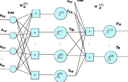
3.1. Iris Dataset
The structure has five input neurons including bias and one output neuron. The results obtained for the proposed algorithm is compared with random weight initialization method and Nguyan-Widrow weight initialization meth-
od and tabulated in Table 1. The learning curve for the
first fold in 10-CV is shown in Figure 2.
The proposed weight initialization method converges quickly with less number of epochs and time. The mini- mum MSE obtained is 0.000353 within 0.1secs whereas the random and Nguyan-Widrow converge to 0.000358 and 0.000356 respectively within 0.2secs and 0.4secs respectively. For all the considered network size the pro- posed weight initialization method converges quickly.
3.2. Two Spirals Problem
[image:4.595.56.288.346.696.2]In this problem, we used 500 input patterns. The points are selected with a radius of 1.5 units. The input coordi- nates represent the points of two interwined spirals in the two dimensional plane. The network is trained to classify
Table 1. Comparison table for Iris data set problem.
Algorithm N/W
Structure Epochs
Training MSE
Validation MSE
Training Time in Secs
Prop + BP
NW + BP
Random + Bp 5-3-1
52
281
220
0.000354
0.000356
0.000361
0.000352
0.000359
0.000362 0.3
0.4
0.4
Prop + BP
NW + BP
Random + Bp 5-7-1
61
261
241
0.000357
0.000358
0.000359
0.000352
0.000359
0.000363 0.2
0.5
0.4
Prop + BP
NW + BP
Random + Bp 5-9-1
89
156
207
0.000355
0.000359
0.000360
0.000351
0.000358
0.000359 0.3
0.6
0.4
Prop + BP
NW + BP
Random + Bp 5-10-1
23
350
111
0.000353
0.000361
0.000358
0.000358
0.000359
0.000360 0.1
1.1
0.2
0 0 . 0 0 1 0 . 0 0 2 0 . 0 0 3 0 . 0 0 4 0 . 0 0 5 0 . 0 0 6
0 2 0 4 0 6 0 8
E p o c h s
MS
E
0
Figure 2. Learning curve based on MSE and epochs of ben- ch mark problem Iris data set for the proposed algorithm.
the points of two separate spirals. The points lying on the spirals are recognized with its corresponding target val- ues 0.1 and 0.9. The network architecture taken for com- parison are 3-8-1, 3-10-1 and 3-11-1 for the proposed weight initialization method, NW weight initialization method and Random weight initialization method. The results obtained are tabulated in Table 2.
The minimum training MSE obtained for the proposed method for the network architecture 3-8-1, 3-10-1 and 3-11-1 are 0.078954, 0.078961 and 0.078950 respec-tively within 1.5, 1.3 and 1.8 secs and 212, 156 and 194 epochs respectively. Similarly for the NW method the minimum training MSE obtained for the network archi-tecture 3-8-1, 3-10-1 and 3-11-1 are 0.078843, 0.078960 and 0.078939 respectively within 2.2, 3.0 and 2.5 secs and 301, 346 and 262 epochs respectively. For the ran-dom initialization method the Training MSE obtained are 0.078982, 0.078833 and 0.078929 respectively within 1.7, 2.6 and 2.4 secs and 242, 295 and 254 epochs respect- tively. From the table it has been observed that the pro-posed method require minimum number of epochs and time for convergence. The learning curve for the first fold in 10-CV is shown in Figure 3.
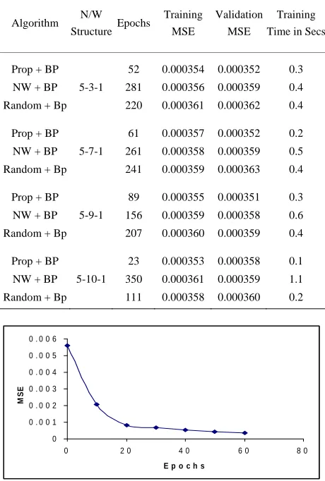
3.3. Modeling a Three Input Nonlinear Function Problem
The nonlinear function is given as follows :
2sin
yz z z
where z3x12x2x3.
[image:4.595.57.287.352.693.2]500 uniformly sampled data from the input range [0,1] are used in this problem. The value of y is normalized in the interval [0.005,0.95]. The simulation results obtained for the proposed method, NW weight initialization meth- od and random weight initialization method is tabulated in Table 3.
Table 2. Comparison table for two spirals problem.
Algorithm N/W
StructureEpochs
Training MSE
Validation MSE
Training Time in Secs
Prop + BP
NW + BP
Random + Bp 3-8-1
212
301
242
0.078954
0.078843
0.078982
0.082371
0.081922
0.082864 1..5
2..2
1..7
Prop + BP
NW + BP
Random + Bp 3-10-1
156
346
295
0.078961
0.078960
0.078833
0.081067
0.082628
0.081947 1..3
3.0
2.6
Prop + BP
NW + BP
Random + Bp 3-11-1
194
362
254
0.078950
0.078939
0.078929
0.081925
0.082281
0.082471 1.8
2.5
[image:4.595.308.538.550.719.2]From the table it is observed that the proposed method performs well in terms of epochs and time for all the net- work structures. The minimum training MSE obtained for the proposed algorithm for the network structures 4- 8-1, 4-10-1 and 4-11-1 are 0.000136, 0.000138 and 0.000137 respectively within 0.9, 0.6 and 0.8 secs-re- spectively. The learning curve for the first fold in 10-CV is shown in Figure 4.
0 . 0 7 8 9 0 . 0 7 9 0 . 0 7 9 1 0 . 0 7 9 2 0 . 0 7 9 3 0 . 0 7 9 4 0 . 0 7 9 5 0 . 0 7 9 6 0 . 0 7 9 7
0 5 0 1 0 0 1 5 0 2 0 0 2 5 0
E p o c h s
MS
[image:5.595.61.284.197.303.2]E
[image:5.595.56.290.373.680.2]Figure 3. Learning curve based on MSE and epochs of two spirals problem for the proposed algorithm.
Table 3. Comparison table for modeling a three input nonlinear function problem.
Algorithm N/W
Structure Epochs
Training MSE
Validation MSE
Training Time in Secs
Prop + BP
NW + BP
Random + Bp 4-8-1
118
224
249
0.000136
0.000136
0.000134
0.000137
0.000137
0.000135 0.9
1.7
1.8
Prop + BP
NW + BP
Random + Bp 4-10-1
68
214
186
0.000138
0.000137
0.000136
0.000139
0.000138
0.000137 0.6
1.9
1.6
Prop + BP
NW + BP
Random + Bp 4-11-1
81
302
216
0.000137
0.000134
0.000136
0.000137
0.000135
0.000137 0.8
3.0
2.1
0 0 . 0 0 0 5 0 . 0 0 1 0 . 0 0 1 5 0 . 0 0 2 0 . 0 0 2 5 0 . 0 0 3 0 . 0 0 3 5
0 5 0 1 0 0 1 5 0 2 0 0
E p o c h s
MS
E
Figure 4. Learning curve based on MSE and epochs of modeling a three input nonlinear function problem for the proposed algorithm.
3.4. Nonlinear Function Approximation Problem
A nonlinear function approximation with 8 input values
i
x is defined in this problem. The three output quantities are defined by the following equations:
i
y
1 1 2 3 4 5 6 7 8 4
y x x x x x x x x
2 1 2 3 4 5 6 7 8 8
y x x x x x x x x
1 23 1 1
y y (13)
500 number of input values are randomly
generated and the corresponding i are calculated using
(13). The network structure considered are 9-10-3 and 9-11-3 for all the weight initialization methods consid- ered for comparison. The termination condition fixed for all the methods is 0.0002. The results obtained are tabu- lated in Table 4.
0, 1i
x y
The minimum number of epochs required for the net-work structure 9-10-3 and 9-11-3 of the proposed method are 427 and 480 respectively and corresponding time re- quired to reach the termination condition is 5.6 and 6.9 secs respectively. Similarly for the same network struc-ture NW weight initialization method requires 780 and 662 epochs respectively to reach the termination condi- tion within 10.5 and 9.4 secs respectively.
For the random initialization method the number of epochs required are 676 and 571 respectively to reach the termination condition within 8.9 and 8.2 secs. The learn-ing curve for the first fold in 10-CV is shown in Figure 5.
3.5. Breast Cancer Dataset
[image:5.595.56.289.374.681.2]The breast cancer data set [23] is one of the best known databases in the pattern recognition literature. The first 250 instances with 30 input attributes are used to diag- nose whether the breast tumors are benign or malignant. Since the original data set varies greatly, they are nor-malized to the range [–1, 1]. The output patterns use 0.1 and 0.9 to represent whether the tumors are benign or malignant. The network structure considered are 31-5-1 and 31-8-1. The results obtained for the proposed method is compared with random weight initialization method
Table 4. Comparison table for nonlinear function approxi- mation problem.
Algorithm N/W
StructureEpochs
Training MSE
Validation MSE
Training Time in Secs
Prop + BP
NW + BP
Random + Bp 9-10-3
427
780
676
0.000198
0.000197
0.000199
0.000221
0.000209
0.000229 5.6
10.5
8.9
Prop + BP
NW + BP
Random + Bp 9-11-3
480
662
571
0.000167
0.000198
0.000198
0.000182
0.000220
0.000221 6.9
9.4
[image:5.595.307.539.607.722.2]0 0 . 0 0 0 5 0 . 0 0 1 0 . 0 0 1 5 0 . 0 0 2 0 . 0 0 2 5 0 . 0 0 3 0 . 0 0 3 5 0 . 0 0 4
0 1 0 0 2 0 0 3 0 0 4 0 0 5 0 0
E p o c h s
MS
[image:6.595.64.284.84.193.2]E
Figure 5. Learning curve based on MSE and epochs of non- linear function approximation problem for the proposed algorithm.
and Nguyan-Widrow weight initialization method and tabulated in Table 5. The termination condition fixed for all the methods are MSE 0.03. The random initialization method require 277 and 272 epochs to converge to MSE 0.028789 and MSE 0.028819 within 1.4 and 2.1 seconds respectively. At the same time NW weight initialization method require 1.3 and 2.5 seconds to converge to MSE 0.028830 and MSE 0.028745 within 256 and 320 epochs respectively.
The proposed method requires 0.4 seconds to reach the minimum MSE within 93 epochs for the network struc-ture with 5 hidden neurons and 0.8 seconds to reach the minimum MSE within 135 epochs for the network struc-ture with 8 hidden neurons.
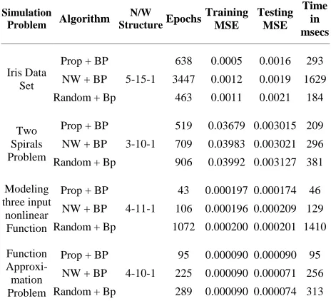
4. Discussion
In order to show the weights obtained by the proposed method are able to reduce the number of iterations, 25 simulations are carried out for the above problems with different network structure and different learning rates. The average number of epochs required to reach the
minimum mean squared error is recorded in Table 6.
Even though the time complexity of the proposed
method is O(n2), it reaches the minimum error in
mini-mum time because it involves linear system of equations and also it is ensured that the outputs of hidden neurons are in the active region before finding the weights for
each layer. From the Table 6 it was observed that the
proposed algorithm required minimum number of epochs and time to reach minimum mean squared error.
5. Conclusions
[image:6.595.306.539.112.231.2]A new weight initialization method using cauchy’s ine-quality based on sensitivity analysis for single hidden layer FNN is proposed. In the proposed method output of hidden neurons are in the active region. The proposed method is simulated on various problems using backpro- pagation learning algorithm. The results are compared with NW weight initialization method and random weight initialization method. From the simulation it is observed
Table 5. Comparison table for nonlinear function approxi- mation problem.
Algorithm N/W
StructureEpochs
Training MSE
Validation MSE
Training Time in Secs
Prop + BP
NW + BP
Random + Bp 31-5-1
93
256
277
0.029165
0.028830
0.028789
0.028220
0.031176
0.031157
0.4
1.3
1.4
Prop + BP
NW + BP
Random + Bp 31-8-1
135
320
272
0.029062
0.028745
0.028819
0.027797
0.031078
0.031168
0.8
2.5
2.1
Table 6. Comparison table for all the problems.
Simulation
Problem Algorithm N/W
Structure Epochs Training
MSE
Testing MSE
Time in msecs
Iris Data Set
Prop + BP
NW + BP
Random + Bp 5-15-1
638
3447
463
0.0005
0.0012
0.0011 0.0016
0.0019
0.0021 293
1629
184
Two Spirals Problem
Prop + BP
NW + BP
Random + Bp 3-10-1
519
709
906
0.03679
0.03983
0.03992
0.003015
0.003021
0.003127 209
296
381
Modeling three input
nonlinear Function
Prop + BP
NW + BP
Random + Bp 4-11-1
43
106
1072
0.000197
0.000196
0.000200 0.000174
0.000209
0.000201 46
129
1410
Function Approxi-mation Problem
Prop + BP
NW + BP
Random + Bp 4-10-1
95
225
289
0.000090
0.000090
0.000090 0.000090
0.000071
0.000074 95
256
313
that the proposed method perform well in terms of time, epochs and mean squared error. Also the proposed method converges very quickly without any flat spot. For all the network sizes the proposed method converges pro- perly without any deviations.
REFERENCES
[1] R. Battiti, “First and Second Order Methods for Learning: Between Steepest Descent and Newton’s Method,” Neu- ral Computation, Vol. 4, No. 2, 1992, pp. 141-166.
doi:10.1162/neco.1992.4.2.141
[2] W. L. Buntine and A. S. Weigend, “Computing Second De- rivatives in Feedforward Networks: A Review,” IEEE Transactions on Neural Networks, Vol. 5, No. 3, 1994, pp. 480-488. doi:10.1109/72.286919
[3] G. B. Orr and T. K. Leen, “Using Curvature Information for Fast Stochastic Search,” Neural Information Process- ing Systems, Vol. 9, 1996, pp. 606-612.
[image:6.595.307.539.269.480.2]ucts for Second Order Gradient Descent,” Neural Com- putation, Vol. 14, No. 7, 2002, pp. 1723-1738.
doi:10.1162/08997660260028683
[5] F. Biegler-Konig and F. Barnmann, “A Learning Ago-rithm for Multilayered Neural Networks Based on Linear Least Squares Problems,” Neural Networks, Vol. 6, No. 1, 1993, pp. 127-131. doi:10.1016/S0893-6080(05)80077-2
[6] Y. F. Yam and T. W. S. Chow, “Determining Initial Weights of Feedforward Neural Networks Based on Least Squares Method,” Neural Processing Letters, Vol. 2, No. 2, 1995, pp. 13-17. doi:10.1007/BF02312350
[7] Y. F. Yam, T. W. S. Chow and C. T. Leung, “A New Method in Determining the Initial Weights of Feedfor-ward Neural Networks for Training Enhancement,” Neu-rocomputing, Vol. 16, No. 1, 1997, pp. 23-32.
doi:10.1016/S0925-2312(96)00058-6
[8] G. P .Drago amd S. Ridella, “Statiscally Controlled Acti- vation Weight Initialization (SCAWI),” IEEE Transac- tions on Neural Networks, Vol. 3, No. 4, 1992, pp. 899- 905. doi:10.1109/72.143378
[9] D. Nguyen and B. Widrow, “Improving the Learning Speed of 2-Layer Neural Networks by Choosing Initial Values of the Adaptive Weights,” Proceedings of the In-ternational Joint Conference on Neural Networks, San Diego, Vol. 3, 17-21 June 1990, pp. 21-26.
doi:10.1109/IJCNN.1990.137819
[10] H. Shimodaira, “A Weight Value Initialization Method for Improved Learning Performance of the Back Propaga- tion Algorithm in Neural Networks,” Proceedings of the sixth Internation Conference on Tools with Artificial In- telligence, New Orleans, 6-9 November 1994, pp. 672- 675. doi:10.1109/TAI.1994.346429
[11] M. Lehtokangas, J. Saarinen, K. Kaski and P. Huuhtanen, “Initializing Weights of a Multilayer Perceptron Network by Using the Orthogonal Least Squares Problem,” Neural Computation, Vol. 7, No. 5, 1995, pp. 982-999.
doi:10.1162/neco.1995.7.5.982
[12] Y. Liu, C. F. Zhou and Y. W. Chen, “Weight Initializa- tion of Feedforward Neural Networks by Means of Partial Least Squares,” International Conference on Maching Learning and Cybernetics, Dalian, 13-16 August 2006, pp. 3119-3122.
[13] X. M. Zhang, Y. Q. Chen, N. Ansari and Y. Q. Shi, “Mini- Max Initialization for Function Approximation,” Neuro-computing, Vol. 57, 2004, pp. 389-409.
doi:10.1016/j.neucom.2003.10.014
[14] M. Fernandez-Redondo and C. Hernandez-Espinosa, “A Com- parison among Weight Initialization Methods for Multi-layer Feedforward Networks,” Proceedings of the IEEE- INNS-ENNS International Joint Conference on Neural Networks, Como, Vol. 4, 24-27 July 2000, pp. 543-548 . [15] T.-C. Hsiao, C.-W. Lin and H. K. Chiang, “Partial Least
Squares Algorithm for Weight Initialization of Backpro- pagation Network,” Neurocomputing, Vol. 50, 2003, pp. 237-247. doi:10.1016/S0925-2312(01)00708-1
[16] M. Huskan and C. Goerick, “Fast Learning for Problem Classes Using Knowledge Based Network Initialization,”
Proceedings of International Conference on Neural Net-works, Como, 24-27 July 2000, pp. 619-624.
[17] D. Erdogmus, O. Fontenla-Romero, J. C. Principe, A. Alon- so-Betanzos and E. Castillo, “Linear-Leaset-Squares Initia- lization of Multilayer Perceptrons through Backpropaga- tion of the Desired Response,” IEEE Transactions of Neu- ral Networks, Vol. 16, No. 2, 2005, pp. 325-337.
doi:10.1109/TNN.2004.841777
[18] Y. F. Yam and T. W. S. Chow, “A Weight Initialization Me- thod for Improving Training Speed in Feedforward Neu- ral Network,” Neurocomputing, Vol. 30, No. 1-4, 2000, pp. 219-232. doi:10.1016/S0925-2312(99)00127-7
[19] Y. F. Yam and T. W. S. Chow, “Feedforward Networks Trai- ning Speed Enhancement by Optimal Initialization of the Synaptic Coefficients,” IEEE Transactions on Neural Networks, Vol. 12, No. 2, 2001, pp. 430-434.
doi:10.1109/72.914538
[20] E. Castillo, O. Fontenla-Romero, A. A. Betanzos and B. Gui- jarro-Berdinas, “A Global Optimum Approach for One Layer Neural Networks,” Neural Computation, Vol. 14, No. 6, 2002, pp. 1429-1449.
doi:10.1162/089976602753713007
[21] E. Castillo, B. Guijarro-Berdinas, O. Fontenla-Romero and A. A. Betanzos, “A Very Fast Learning Method for Neu- ral Networks Based on Sensitivity Analysis,” Journal of Machine Learning Research, Vol. 7, 2006, pp. 1159-1182. [22] R. A. Fisher, “The Use of Multiple Measurements in Taxo- nomic Problems,” Annual Eugenics, Vol. 7, No. 2, 1936, pp. 179-188. doi:10.1111/j.1469-1809.1936.tb02137.x
[23] A. Frank and A. Asuncion, “UCI Machine Learning Re- pository,” School of Information and Computer Science, Universty of California, Irvine, 2010.