A Review of Active Learning and Co Training in Text Classification

A Review of Active Learning and Co-Training in

Text Classification

Michael Davy

Machine Learning Group

Department of Computer Science

Trinity College Dublin

November 4, 2005

1

Introduction

Ever increasing volumes of data in electronic format are being produced and stored, due mainly to the relatively inexpensive cost of storage and emerging techniques for extracting useful information from such data. A large corpus of data, in itself does not offer a lot of value but if it were categorised into relevant, prescribed categories, this data could become quite useful.

Text classification is the name given to automated techniques for grouping textual information into categories. The task of categorisation lends itself fully to automation. Large corpora of data require administration and a technique to effectively manage the data, since the rate at which data is produced is far in greater that the rate at which it can be manually processed. Manual cate-gorisation of data is feasible only in the small scale. Even a small organisation can now produce large amounts of data.

Modern machine learning techniques (supervised learning) allow for a classi-fier1to be produced using only labelled examples from concept that is required to be learned. Previously, considerable human effort was required to manually construct and maintain hand-crafted rules which formed the classifier. Modern machine learning techniques has allowed for off the shelf learners which given enough training data can construct an accurate classifier.

Large quantities of training data are required for an accurate classifiers to be produced. However, obtaining labelled training examples can often be an expensive task in itself. Typically, examples need to be manually labelled which is a laborious, time consuming and repetitive task. Most humans do not relish the idea of labelling thousands of examples.

In many domains labelled training data is either scarce or expensive to pro-duce. Unlabelled data, on the other hand, is plentiful and inexpensive to collect. The learner should make use of this unlabelled data to help it produce an ac-curate classifier without the need for large amounts of labelled training data.

Active learning and Co-Training are methods which require very little la-belled training data and exploit unlala-belled data in order to increase accuracy

of a produced classifier. Both are employed at the initial stages of a learner’s life-cycle and are iterative in nature.

Active learning is a term used to describe a learning method whereby the learner assumes (some) control over the training data. This differs from the tra-ditionalpassive learning, indicative of supervised learning, whereby the learner has no control over the training data. An active learner makes use of an external teacher (an oracle) which will label a presented example correctly thus produc-ing more trainproduc-ing data. It is the task of active learner to select and present to the oracle, the most informative cases which will maximise learning.

Co-Training is a process which uses multiple views of the same data to boost classifier accuracy. A view is simply a way to describe the data, for example an e-mail can be described by both the header and the body information. The learner will exploit nuances in each view to help it automatically label those unlabelled examples which its classifier has predicted with high confidence -which then becomes new training data.

There are many domains in which machine learning could be applied but is not due to the lack of labelled training data. Methods such as Active Learning and Co-Training allow machine learning solutions to be applied to new domains previously thought to be unsuitable for machine learning solutions. These meth-ods also have an impact for traditional machine learning domains. Productivity could increase as more tasks that should be automated (but are not due to scarcity of training data) are solved using machine learning techniques com-bined with active learning and co-training.

The rest of the paper is organised as follows. Section 2 describes Active Learning and the various different approaches used to select unlabelled exam-ples. Section 3 describes Co-Training and also its merger with active learning, namely, Co-Testing. In Section 4 we discuss our conclusions and future work. We start, however, with a very brief review of Text Classification.

2

Text Classification

Text classification 2 can be defined as assigning categories to textual units of data. As the production of data increases, the adoption and use of text classi-fication systems needs to also increases in order to help humans deal with the large volumes of data. This can be seen in scenarios whereby large corpora of business documents are being categorised allowing humans to make more specific searches and navigate the information easily. Another role is that of filtering, whereby a classifier learns a specific user’s preference and filters out information that would be deemed irrelevant. Thus the user views only relevant and precise information leading to increased productivity.

A brief history of machine learning and its adoption into real world applica-tion is given below, followed by an overview of the text classificaapplica-tion architecture. This section gives only a brief overview. For a full discussion on all the topics related to text classification please consult [Seb02].

2.1

Text Classification History

In recent years the adoption of machine learning into modern complex systems has seen a dramatic increase. The main reason for this is that it often works very well. The examples presented in [LMF+04] show that given the correct domain and sensible requirements, machine learning can produce very useful systems.

Expert systems were among the first applications to be used in the real world. More recently, data mining has become very popular because it can allow the extraction of potentially useful (business) logic from dormant data that has been collected over time.

Information retrieval has grown prominent in recent years, mainly due to the meteoric popularity of the internet. It is concerned with the retrieval, storage and extraction of information from documents.

Text classification can be defined as: “the activity of labelling natural lan-guage texts with thematic categories from a predefined set” as given in [Seb02]. This differs from information retrieval but a lot of common ground exists. In-deed many techniques of text classification are taken from the work done in information retrieval.

2.1.1 Knowledge Engineering

One of the first approaches was that of Knowledge Engineering, commonly known as Expert Systems. Expert systems are constructed by domain experts manually constructing and configuring a set of rules in the form of:

if (condition) then (classification).

The condition was normally concerned with some attribute of the example pre-sented to the system (e.g. if the document contained the word ‘wheat’). If and only if, the conditions were met in the rule then the classification would be assigned to the instance. These systems performed well, but they suffer from the problem ofknowledge acquisition bottleneck, which refers to the high cost in defining and maintaining rules for the system. The initial cost is extremely high as analysis of the domain and domain experts are required in order to construct the rules within the expert system. Moreover the costs associated with chang-ing the system over time, as the role or requirements of the system changes, are also extremely high, due to the fact that domain experts are again needed to construct an updated set of rules. If the system is legacy then it may be necessary to train personnel to become domain experts before the system can be updated.

than junior doctors, but included a certainty factor which allowed doctors to determine whether or not to accept the decision of the system. Big business has also adopted such systems with dramatic affects, the R1 expert system [McD82] developed for the Digital Equipment Corporation. It’s role was to configure orders for new computer systems and was estimated at saving the company $40 Million. Soon practically every large company or organisation was investing in expert systems. In more recent times, knowledge engineering has been used in the fight against spam. Systems such as Spamassassin use a list of rules, which are updated at regular intervals, to filter out spam from legitimate e-mail (in fact Spamassassin has also incorporated a machine learning approach also).

Knowledge engineering does offer very good performance and accuracy but it does have drawbacks. As mentioned previously the knowledge acquisition bottleneck is perhaps its most serious flaw. These systems are very domain specific, that is, they can not easily be ported to another domain. For example, the MYCIN system could not easily be ported to look at astronomical images for detection of meteorites. It would require considerable cost and effort to update the rules in order to comply with the new requirements. This is whereMachine Learning methods show their strength. Machine learning is roughly defined as: “the ability to adapt to new circumstances and to extrapolate patterns”. The important point to note here is the ability to adapt to new circumstances.

2.1.2 Machine Learning Approach

Rather than focusing on developing domain specific systems, researchers began to focus on developing a way construct a system which could work in any do-main. Machine learning approaches allowed for rules to be constructed from a set of labelled training examples. This allowed for a generic algorithm to be developed, where it would construct a domain specific classification system based on series of labelled training examples (collectively known as training data) given as input. This relieves the knowledge acquisition bottleneck since domain experts are no longer consulted and only training data is needed for a system to be produced. However, as is noted in [LMF+04], training data needs to be carefully constructed. Using poor or noisy training data can result in a system which fails to meet some or all of the requirements since the training data used as input do not reflect the unseen instances from the domain.

Since the task of labelling a set of training examples is far easier than that of constructing precise and robust set of rules, the number of areas and applications incorporating machine learning has grown. However, for an accurate classifier to be constructed, a large number of training examples are needed. This is bounded by PAC learnability which stipulates a minimum number of examples needed in order to have a bounded error on accuracy. Discussion of PAC learnability is outside the scope of this document, for more information on this topic please consult [Mit97].

retrieval of relevant information.

2.2

Types of Learning

Text classification is concerned with assigning predefined labels to documents by means of a functionf. This is accomplished by inductive learning, that is, learning a hypothesis 3 (h) based on examples or observations of an unknown real world function (f).

There is a number of different learning strategies in which a learner is ex-pected to learn. Some are just given a list of examples and exex-pected to learn some general rules from these. Others are even more neglected and are just given unlabelled examples and expected to learn some rules from this data. There are three main types of learning:

Supervised Learning is where the learner is supplied with exemplars of the form x, f(x) where f(x) is the label assigned by the unknown target function for the instancex. From the training examples the learner con-structs hypotheses (h) which are consistent with the training exemplars. The hypotheses spaceH is the collection of all consistent hypotheses. In-duction is then the task of returning a functionh∈H that approximates f. A good hypothesis is one that will generalise, that is, it will predict unseen examples (x) correctly.

Unsupervised Learning is concerned with identifying classes or labels within a set of data. The input is just a collection of instances from the domain, which have not been labelled by the unknown target functionf(x). This method is useful in the context of text classification when trying to clus-ter instances. It is not discussed in detail in this paper, for a complete background see [Mit97] [Seb02].

Reinforcement Learning is primarily concerned with how a learner interacts with its environment. Actions which the learner conducts are rewarded or punished. The learner can build up an internal representation of its environment which may help it achieve its goal. Reinforcement Learning has seen most use in robotics and computer vision.

For the rest of this paper, we will concentrate on supervised learning as it is most applicable to the realm of text classification. In the text classification scenario, sufficient training data (documents from a domain along with their correct classification) is given to the learner, where it induces a hypothesishthat approximates the unknown target function for the domainf. The hypothesis hcan then be used to classify new and previously unseen documents that are presented to the system.

2.3

Passive Learning

Modern machine learning typically happens in what we call a passive learning scenario. That is the learning machine (the learner) does not participate in-teractively with the teacher. Examples of the task which we wish the learner

to learn are provided but after that no other stimulus is given. In this sec-tion we discuss the different aspects of the passive machine learner starting by explaining what we call a learner.

2.3.1 The Learner

The notion of alearner is often presented in the literature. A learner encapsu-lates the process of inducing a classifier. The learner is given training data and from it produces a classifier. The more traditional notion of a learner is that of a passive learner whereby the learner induces a classifier based on just the training data. There are other types of learner (such as an active learner) that do more with the training data before inducing and output a classifier.

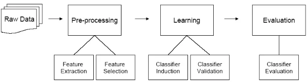
2.3.2 Text Classification System Life-Cycle

Figure 1 is a generic life-cycle for a text classification system. Raw data is given as input. The system needs to convert from the raw data into a notation it can use and manipulate. Typically this is thevector space model which is described in more detail in subsequent sections. Transforming the raw data is done in the pre-processing stages which include feature extraction and feature selection. Once the data is in a useable format, the system can induce a classifier, which is used to classify new and unseen instances. Validation may be performed in order to fine-tune the classifier. Hopefully the classifier should be a good approximation (or indeed equivalent) to the real target concept.

Figure 1: Text Classification System Life-Cycle.

Of course, there is a lot happening in each stage. In the sections that follow processed from each stage are elaborated, giving the reader sufficient under-standing for the rest of the topics raised in the paper. A full discussion of the multitude of different approaches in each stage of the text categorisation system is outside the scope of this document.

2.4

Preprocessing

applications, training data is very limited. It is comprised of a subset of the domain (of lengthm), for which their corresponding category labels are known.

{d1, c1,d2, c2 . . .dm, cm}

d⊂Domain c∈Range

Training data is critical for the success of a classification system, given bad training data the accuracy of the system may be dramatically diminished.

A number of standard benchmarks are used in text classification systems, the most notable addition being the news wire data such as the Reuters corpora. An important recent addition is that of the Enron corpus [KY04]. This may prove to be a valuable resource since it contains a large quantity of real users e-mail together with classification done by the users into folders. Finally the UCI repository contains a large collection of data sets which can be used, while not specifically text classification data, these can still be useful for testing and evaluating the separate, constituent parts that form a text classification system.

2.4.1 Feature Extraction

The first stage in pre-processing is that offeature extraction. A feature can be any piece of information known about a document, these include the individual words within the document (known astokens) or non-token features such as the size of the document. Establishing a coherent and descriptive set of features is vital for a successful text classification system. Unless we can extract mean-ingful information from documents the system may not perform accurately or efficiently. Each state of each document can then be represented as a vector of N features, whereN is the number of unique tokens in the entire collection of documents.

d_i=a1, a2, a3. . . aN

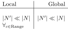
2.4.2 Feature Selection

Even for the most trivial of tasks, N can grow to be extremely large, making searching this state space of all documents infeasible. Using feature selection

the dimensionality of the state space can be significantly reduced allowing for efficient searching. There are two possible ways to conduct feature selection:

local, where we do feature selection with respect to each categoryc∈Range or

global, where feature selection is done with respect to all categories.

Local Global

|N| |N| |N| |N|

∀c∈Range

There are a number of methods that are widely used for feature selec-tion, these includeInformation Gain[SW48] and the method which shows most promise Latent Semantic Indexing (LSI)[DDL+90]. While the latter does seem to produce better results, patent issues associated with it have stunted its wide scale adoption.

2.5

Learning

At this stage the data has been transformed from its raw state into a model which can be easily processed. In addition the demensionality of this model has been reduced to make it more managable. A classifier can now be constructed from this data.

2.5.1 Classifier Induction

Inductive learning is concerned with learning from examples about which class membership is already known. An inductive learner will induce a hypothesis (h) that will approximate the target function (f) as much as possible.

The goal of a text classification system is to find a function that will map all the documents in the domain to the correct classification in the range. This ideal function is called the target function. Text classification systems, given enough correctly labelled examples, will deduce hypotheses based on the exam-ples. There can be numerous hypotheses that satisfy all the training examexam-ples. The collection of all the hypotheses that satisfy the training data is called the version space[Mit97]. In Machine Learning, the target function is considered to be within a version space, the goal is then to either find the target function by searching the version space. Inductive learning is concerned with learning from examples about which class membership is already known. An inductive learner will induce a hypothesis (h) that will approximate the target function (f) as much as possible.

There are two main types of classification problems, namely, multi-class and binary. The majority of the research has concentrate on binary classification problems, that is, the total number of possible labels is two (for example,f(x) = y, y ∈ {spam, legit}). The reason for concentrating on binary classification problems is that multi-class classification problems can be decomposed into a series of binary classification problems.

The output from the pre-processing stage typically results in a number of training examples (fori= 0. . . M whereM is the number of training examples), each represented by a feature vector (d_i) and an associated classification label (y_i).

d_i=a1, a2, a3. . . aN

f(d_i) =y_i

Scut involves testing different values for the threshold using a validation set and choosing a value which maximises the effectiveness of the classifier. With Scut there will be different thresholds for the different categories. Rcut is simply where a fixed threshold is used. Pcut, as described in [Seb02], is when the value of the threshold is chosen so that the generality of the training set gtr(yi) is closest to the generality of the validations setgV s(yi), that is the same percentage of documents, for both the training and validation set, are classified under categoryyi.

gΩ(yi) = |{dj∈Ω|h(dj, yi) =T|

|Ω|

2.5.2 Types of Classifier

While a full enumeration of all inductive classifiers is beyond the scope of this paper, a brief discussion will be given on some of the more popular and inter-esting classifiers seen in text classification systems.

Perhaps one of the most widely used classifiers is the na¨ıve Bayesian classifier. It is a probabilistic classifier, thus it produces hypothesish(x) =y where y = [0,1]. It uses the training data to construct conditional probabilities which are used to infer probabilities about the classification of future instances presented to the learner. The na¨ıve part stems from the independence assumption, which assumes that features are conditionally independent. In reality this is not the case but this assumption simplifies the calculations significantly. Please consult [Mit97] for a full discussion on Bayesian classifiers.

y_NB=arg max_yi∈YP(y_i)

j

P(a_j|y_i)

Thek Nearest Neighbour (kNN) is a memory based classifier, called so as it keeps in memory all the training examples. It does not do any processing during training, rather it does its processing during classification. For this reason it is called a lazy learner. As an instance is presented to the learner, it will search through its memory looking for examples which are similar to the instance presented to it. It will then select the k training examples that are most similar and use these to determine the classification of the presented instance. Similarity is normally measured in terms of Euclidean distance, while a majority vote (or the mode of the classification) of the training examples is used to determine the classification. Because of its simplicity and ease of comprehension, kNN is a widely used classifier.

Decision trees are called symbolic learners which humans find easier to comprehend. They construct a tree in which internal nodes are features and branches departing from these nodes represent the values associated with the feature. Leaf nodes correspond to categories in the classification task. There are numerous algorithms for constructing decision trees, the more popular are ID3 and C4.5. A divide and conquer strategy is used in the construction of a decision tree, in which the feature which best splits the data into categories are chosen as nodes in the tree. Clearly quite large trees can be produced which can also overfit. Pruning can be done with a validation set in order to reduce the size and help generalise the decision tree.

correctly. If this can not be achieved in the original feature space, instance can be mapped into a higher dimension feature space where the instances are linearly separable. This is done using a kernel method. For a full description of support vector machines please consult [Vap98].

Linear (also known as an On-line) classifiers produce a classifier almost im-mediately after examining the first training example, which is in contrast to batch classifies (like the ones above) which examine the entire training set be-fore inducing a classifier. They receive examples one at a time and incrementally refine the classifier. These refinements are characterised by additive and multi-plicative update algorithms.

2.5.3 Committee Based Classifiers

Committee based classifiers (also known as an ensemble) combine the predictions of multiple classifiers in order to increase accuracy. A committee is characterised by the choice of the constituent classifiers and on how to combine the predictions of the individual classifiers into one overall classification. Diversity is essential for a committee [MM03]. The easiest way in which to combine the predictions of the individual classifiers is that of majority vote. Alternatively a weighted vote can be done where each classifier is assigned a weight based on its expected relative effectiveness. Dynamic classifier selection is where the classifier which was most accurate on examples encountered during training that are similar to the presented instance, is selected as the classifier that will produce the overall classification.

There are two main approaches to producing ensembles, bagging and boost-ing. Bagging is a re-sampling technique used to construct an ensemble. Several bootstrap samples are drawn at random, with replacement, from the training set. Each sub sample is then used to train a single classifier which then becomes a constituent member of the ensemble. A majority voting scheme is normally used to give an overall classification.

Boosting is a technique for constructing an ensemble in a sequential process, where extra attention is given tohard to classify examples. In this way subse-quent classifiers produced during the boosting procedure can incorporate knowl-edge about how previous classifiers performed. Each training example is given a weight according on how difficult it was to classify (i.e. based on previous classifiers misclassifying it). Similarly to bagging, boosting randomly selects samples from the training set, with replacement, except instead of assuming a uniform distribution like in bagging, it will perform weighted sampling using the weights assigned to each training example. The idea is that more difficult to classify examples will be more likely to be selected. The most prominent boosting technique is AdaBoost [Sch99].

2.6

Evaluation

The performance of a text classification system is measured empirically using a variety of standard metrics borrowed from other fields such as information retrieval.

negative (i.e. not belonging to a category). False negative refers to the case where the classifier incorrectly identifies a positive case as being negative. False positive refers to the case where the classifier incorrectly identifies a negative case as being positive.

In some scenarios the costs associated with each of these are equal while in others scenarios the cost of a false positive far outweighs the cost of a false negative, as is the case in the spam filtering (getting a few spam in your inbox is bearable, but loosing an important e-mail because it was marked incorrectly as spam is disastrous).

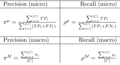
Precision and Recall, which are used in information retrieval, can be defined as follows.

Recall(ρ) = T P T P+F N

P recision(π) = T P T P+F P

There are two different approaches to calculating precision and recall, which are micro averaging and macro averaging. In the micro case, the values for TP, TN, FP and FN are computed per category and are then combined for an overall figure of precision and recall. In the macro case, the values of precision and recall are computed in each category and then these values are averaged to give an overall value.

Precision (micro) Recall (micro)

πµ=

|C| i=1T Pi

|C|

i=1(T Pi+F Pi)

ρµ =

|C| i=1T Pi

|C|

i=1(T Pi+F Ni)

Precision (macro) Recall (macro)

πM =

|C| i=1πi

|C| ρM =

|C| i=1ρi

|C|

Table 2: Formulas for calculating the Micro-Averaged and Macro-Averaged precision & recall values.

Micro averaging gives equal weight to each document while macro averaging gives equal weight to each category.

The breakeven point is the value at which precision equals recall (π =ρ). While the F_β measure is a way of combining precision and recall into a single value for easier comparison.

Fβ= (β

2_{+ 1)πρ}

β2π+ρ

Typically β= 1 which means that there is equal importance to both precision and recall, where as ifβ= 0 then all importance is given to precision. Similarly ifβ= +∞then all importance is given to recall.

Accuracy is defined as.

while error is defined as.

Error= 1−Accuracy

If accuracy is used in parameter tuning validation, the classifier may behave like a trivial rejecter. This is due to the fact that a large denominator makes it insensitive to changes in TP and TN which is not the case with precision and recall.

3

Active Learning

A general principle in machine learning is that the more training data a learner has, the more accurate it should be. This stems from PAC learnability, which tries to measure how many training examples are required for a learner to achieve a bounded error rate. From PAC learnability it is safe to deduce that the more training data given to the learner the more accurate the model produced by the learner should be (in other words, more consistent with the target concept). The reason why, in practice, machine learning classifiers are trained with very large amounts of training data is due to the fact that not all examples are equally informative, some possess little to no information value while others are extremely informative. Thus the larger the training dataset the higher the probability that the training data contains the minimum number of informative training examples (as described by PAC learnability) needed by the learner in order to induce an accurate classifier.

In most domains there is an abundant amount of raw unlabelled data avail-able. Considerable effort is needed in order to construct a training dataset from which a passive learner can induce a hypothesis consistent with the tar-get concept. A large number of examples must be labelled in order to produce the training dataset. In some cases the effort in constructing a large training dataset is prohibitive. The reason may be that the training data is very limited or extremely costly to acquire (for example an expensive blood test). It would be very beneficial if we could reduce the size of the training dataset without impacting on accuracy of the classifier learned.

Active learning allows for a dramatic reduction in the size of the training dataset needed by a learner. The reduction in the number of labelled training examples is possible by giving the learner more control in the choice of the examples in the training data. The learner typically has a large training dataset but has not control in the choice of the training data.

The active learner can present queries to an oracle, where a query is a case from the domain for which the learner does not know the label. The oracle which is considered a domain expert has the task of correctly labelling the presented query. These queries are the crux of the active learning framework and allow the learner a way to control the training data it uses. Queries can either be constructed by the learner or selected from a source of unlabeled queries.

with fewer training data. This reduces the number of labelled examples needed in order for the learner to find a hypothesis consistent with the target concept. In other words, the non-informative examples are removed from the training data.

The oracle, typically a human that is a domain expert, is a vital part of the active learning framework. Its role is to supply correct labelling to the queries presented by the learner. Since there is a human-in-the-loop, the learning task changes from a batch process to an interactive process. It is assumed that the oracle is infallible thus the labels it provides are indeed correct. This is an important fact since this implies that the training data contains no noise. In the literature the oracle is commonly referred to as a teacher, in this paper oracle and teacher are used interchangeably.

As active learning is an interactive process there is a clear question on how to decide the stopping criteria. An obvious stopping criterion is the number of labellings the oracle is willing to make. Another way of deciding when to stop is to examine the accuracy obtained in each iteration and stop if the accuracy falls. The stopping criteria are still an open issue in the literature.

In this chapter we begin by outlining the differences between passive and active learning. A simple comparison between the two is presented. Next our attention turns to the structure of an active learner. This describes the processes that happen and in what order. Finally we consider how an active learner choosesinformativeexamples. As we will see later this is crux of active learning and several approaches have been tried.

3.1

Active versus Passive Learning

There are two different types of learner, passive and active. The two really differ on how much training data they receive and on how much control they have over the choice of the training data. Both types of learning also use exactly the same machine learning classifiers but differ in the way they induce the classifiers (active learning induces a classifier after each interaction with the oracle). Of the two, passive learning is by far the more straight forward and easier to implement.

3.1.1 Passive Learning

The term passive learning is used to describe a learning algorithm which has no control or influence over the training data it receives as input. This is the most common approach for supervised machine learning algorithms. In these learners there is no oracle; rather the learning is fully automated in a batch process. These learners require a large training dataset in order to produce an accurate classifier. This is because the training dataset may contain a number of non-informative training data.

3.1.2 Active Learning

oracle is assumed to be infallible for the sake of simplicity. Rather than being a batch type process, active learning is somewhat interactive and incremental in nature. Each iteration consists of the learner interacting with the oracle. The learner presents a query to the oracle which then labels the query thereby producing a new training example. This new example is added to the training dataset and a new classifier is induced using all the training dataset.

A number of classifiers are produced during active learning. The final clas-sifier can either be an ensemble of these clasclas-sifiers or can be a clasclas-sifier based on all the labeled training dataset once a stopping criterion has been met.

The goal of an active learner is to achieve comparable levels of accuracy (from a reduced number of training data) with that of a passive learning. Equally, it can also be seen as trying to achieve the highest possible accuracy using all of the (limited) training data. The former goal is more applicable to most scenarios where active learning is used.

3.1.3 Comparison

By its very nature, active learning requires less training data than a passive learner. The point that makes active learning interesting is the fact that the reduction in the size of the training dataset can be of several orders of magnitude! On the other hand, active learning normally requires a lot more resources than passive learning in the form of an oracle and increased complexity in im-plementation issues. There is a need to weigh up the costs of labelling data manually or employing an active learning strategy. If the later is more expen-sive then there is no point in deploying such a system.

By far the most important difference between the two methods is in how much control they can influence over the training examples used to train clas-sifiers. Passive learning exerts absolutely no control; the examples used are selected by the end-user. Active learning does have some influence, ranging from the ability to construct an entirely new example itself, to selecting exam-ples from a pool of unlabeled examexam-ples.

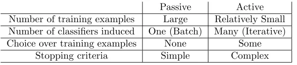
Passive Active Number of training examples Large Relatively Small Number of classifiers induced One (Batch) Many (Iterative) Choice over training examples None Some

Stopping criteria Simple Complex

Table 3: A simple, high level comparison between passive and active learning

3.2

A Generic Active Learning Structure

There is a question of how exactly the process of active learning happens and in what order. Amongst all the different implementations in the literature, a generic structure can be extracted. This structure is meant as a representation of an active learner and not a definitive structure that an active learner should adhere to. Its goal is to help in understanding the processes and sub-processes that happen during active learning.

Given:

Training datasetLof labelled examples OracleT

Source of unlabeled examplesU Stopping criteriaM.

While stopping criteria not met

- Obtain queryxfor Teacher to label.

- Have the Teacher label the queryy=T(x).

- Add example to set of labelled examplesL=L{(x, y)}. - Induce new classifier from training datasetC_i=I(L).

Output a final classifierC

Figure 2: Generic Active Learning Structure

Presented in Figure 2 is a generic structure for an active learner. A number of items are required before active learning can proceed. The definitions of these items given here are deliberately abstract. More concrete definitions are given later when we discuss the different aspects of active learners.

First and foremost the active learner needs a source of unlabeled examples U. Second, it requires a place to store the labeled training dataL. To label the examples, an oracleT (commonly referred to as a Teacher) is required. Finally, a way of knowing when to stop active learning is neededM.

The procedure is as follows; obtain a query that we want the oracle to label. These queries should be very informative. Once obtained, we present these to the oracle which will correctly label them. Placing the newly labeled examples into training dataset, we then induce a new classifier based on the training dataset (and possibly the unlabeled examples also). We keep doing this until the stopping criterion is met.

3.3

The Oracle

Let us firstly discuss the one aspect of the structure which does not seem to change amongst implementations. The teacher or oracle is generally not dis-cussed in the literature. If it is mentioned then it is almost always assumed to be a human. The active learner assumes the presence of an external oracle. The oracle is willing to correctly classify queries presented to it and it can be as-sumed that the oracle is infallible, thus it is not a source of noise in the training data.

The oracle operates in a query-response manner whereby the learner can query the oracle with a particular query and it will return the correct classifi-cation for the query. In many cases the oracle is a human but it could equally be an additional test (for example additional expensive blood tests) which, if conducted, would supply the correct classification.

In [Tur00], cost associated with the oracle is discussed. Turney describe that a “wise learner is one which will classify easy cases by itself and reserve difficult cases for the teacher”. Thus a rational learner would, for each new case pre-sented to it, calculate the cost of classifying the case by itself (misclassification cost) versus the cost of asking the oracle to classify the example.

There is an assumption that the oracle has a cost associated with it. It is necessary to decide whether a misclassification is more expensive than asking the oracle. A form of cost benefit analysis is needed in order to determine when the valuable resource (i.e. the oracle) should be consumed. If the cost of asking the oracle is too high then the learner may never ask a query. On the other hand, if the cost of asking the oracle is too low then the learner may ask numerous trivial questions causing frustration in the oracle.

There is the idea of punishing the learner for asking trivial queries while rewarding the learner for querying difficult and complex examples. Punishment does not seem to be a common approach at present in active learning although it does have some form in reinforcement learning where the agent is punished for making the wrong decision.

One final consideration about the oracle is the way in which it answers queries. The oracle can be configured in one of two ways, the first being that when presented with a query the oracle will return the correct classification for that particular query. The second configuration is that the oracle can return a set of counter examples [Ang88] for each query presented to it. Of the two configurations the former is the more practical and popular.

3.4

Query Sources

Active Learning requires a source of queries. Queries take the form of an unla-belled example, that is, a case for which we do not know the label. The question of where these unlabeled examples come from has created a number of divisions in the active learning literature.

other form is that of a stream from which the learner can extract unlabeled examples. This is referred to as stream based query selection. Of the various sources the pool based query selection is the most popular. Figure 3 shows the hierarchy of queries.

Query

Construction Selection

Pool Stream

Figure 3: Different Types of Queries

3.4.1 Query Construction

One way in which to obtain queries is to have the learner construct its own. Queries can contain any information as long as they conform to the input space. The learner can then find the membership of this constructed query. This comes from a method of learning calledquery learning that was proposed by [Ang88]. An accurate classifier can be constructed from fewer training data if the learning algorithm is allowed to create artificial examples, often called ’queries’ [Ang88]. The learner explicitly constructs the query that will be presented to the teacher. In each of the iteration of active learning the learner will construct an example that conforms to the input space (the domain) and request its label. In this way the learner can exploit its knowledge of the domain in order to construct queries from a region of the input space that it has little knowledge about.

This method has the advantage of utilising the learner’s internal knowledge in order to construct informative queries which should further dramatically in-crease the learner’s knowledge of the domain. However, certain problems arise when constructing such queries, the most notable being that constructed queries are sometimes nonsensical. This is important since the oracle is often a human, thus if they can not understand the query they can not correctly label it. This problem is particularly prevalent in the case of text based domains. Constructed queries are often nonsensical as shown in [BL92].

3.4.2 Pool Based Query Selection

Given

- pool of unlabeled examplesU - set of labeled examplesL

- classifier induction algorithmAwhich will produce a classifierC_t

- example selection functionQ

- oracle T that returns the correct label y for example x such that y=T(x)

while stopping criteria is not met

- UseQto select the most informative examplex. x←Q(U)

- Present the example x to the oracle and obtain the correct label y=T(x).

- Remove the example from the set of unlabeled examplesU. U ←U\ {x}

- Add the newly labeled example to the set of known labeled examples. L←L{(x, y)}

- Induce a new classifier C_t←A(L).

Output: Final classifier(s)C1. . . Ct.

Figure 4: Pool Based Active Learning Structure

We can modify the generic structure of an active learner presented in Figure 2 to reflect a generic pool based query selection active learner structure as given in Figure 4. The learner will select queries from the pool of unlabeled examples with the aim of selecting a query that will maximise the knowledge obtained from knowing the label of this one query. Another way to look at this is that the learner wishes to find the query that will reduce the hypothesis space the most - thus eliminating the hypothesis that are not consistent with the target concept.

The query is chosen using a query selection function. It is the responsibility of this function to select the most informative queries. The query will then presented to the teacher where it is given the correct label. Once the correct label is known the query becomes a training example, whereby it is added to the training dataset. The query is also removed from the pool of unlabelled examples. Finally the learner induces a new classifier based on all the training data in the training dataset.

Clearly the improvement in accuracy is gradual, as the number of training data increase so too should the accuracy of the induced classifier and a reduction in generalisation error. Typically in each run of active learning one example is selected but for reasons of optimisation, multiple examples can be selected in each phase.

Clearly the query selection function is vital for the success of active learning. The function should pick the most informative query from the pool in order to improve the performance of future classifiers. There have been numerous ways suggested in the literature about how to select the next example. We discuss some of the various methods in a later section (3.6).

There are some advantages that pool based selection has advantages over constructed queries. Clearly in the case of text problems the main advantage is that the queries presented to the oracle are existing cases (documents etc. . . ) from the domain. These are comprehensible to the oracle thus a correct label can be assigned.

3.4.3 Stream Based Query Selection

In a slight variation of pool based query selection, stream based selection re-places the pool of unlabelled examples with a stream, from which the learner can draw examples from. The learner has no control over the stream other than the ability to draw examples from it. It is assumed the stream will present examples which are indicative of the underlying distribution in the domain.

This method is more suited to an on-line system, for example an e-mail routing system. At distinct time intervals new instances arrive. The learner will draw the example from the stream where upon it has two choices. It can decide to classify the instance itself or ask the oracle to label it. Typically the learner will decide classify examples for which it has a confident classification. Similarly it will decide to ask the oracle to label the example if its does not have a confident classification.

Once again the learner must do a form of cost benefit analysis to make the decision. If the cost of misclassification is very high, then the system will tend to ask the oracle to label many examples. On the other hand if the cost of labelling by the oracle is high then the cost of misclassification will tend to be more acceptable, thus accuracy may suffer.

Similarly to the generic pool based structure presented in Figure 4, we can modify the generic active learner structure of Figure 2 to reflect a generic struc-ture of a stream based active learner as shown in Figure 5.

In this case, the source of unlabeled examples is given by a streamS. The learner will sample from this stream; for an example which the current classifier is confident about, the learner will decide to label itself and for an example which the current classifier is not confident about, the learner will present to the oracle for labelling.

The remaining structure of a stream based active learner is the same as a pool based active learner. The newly labelled query is added to the training dataset and a new classifier is induced based on all the training data in the training dataset.

disad-Given

- stream of unlabelled examplesS - set of labeled examplesL

- classifier induction algorithm A which will produce a classifierC_t

- teacher T that will return the correct label y for an examplexsuch that y=T(x)

while stopping criteria is not met

- Remove examplex from StreamS about which classification is not confident.

- Present the examplexto the teacher T and obtain the correct label y=T(x).

- Add the newly labelled example to the set of known labelled exam-ples.

L←L{(x, y)} - Induce a new classifier

C_t←A(L).

Output: Final classifier(s)C1. . . Ct.

Figure 5: Stream Based Active Learning

vantage of the learner not being able to examine all unlabelled examples when trying to select the most informative query. In addition, the classifiers induced depend on the sequence of examples in the stream - this may make experiments difficult to replicate or cause instability in an active learning scheme.

3.5

Query Construction Methods

An accurate learner can often be constructed from fewer examples if the learn-ing algorithm is allowed to create artificial examples, often called membership queries [Ang88]. This is where the learner explicitly constructs the query that will be presented to the teacher at each phase of the active learning life-cycle. On each phase the learner will construct an example from the input space (the domain) and request its label.

Certain problems arise when constructing examples, the most notable being that constructed queries are sometimes nonsensical to human observers. This is important since the teacher is often a human. Particularly in the case of text, constructed examples are nonsensical as shown in [BL92].

3.5.1 SGnet

In [CAL94] a region of uncertainty in the domain is identified and unlabelled examples from that region are sampled. While not specifically constructing queries, the method does select examples from the entire domain, thus we are not dealing with a pool based approach. In addition the learner has control over which examples it will select from the domain thus it is not a stream based approach.

The region of uncertainty is defined as consisting of the unlabelled examples from the input domain for which there is a disagreement amongst the consistent concepts in the version space[Mit97]. For a given inputx, and conceptsc_ic_j∈C whereC is the version space consisting of all the concepts which are consistent with the training data. c_i(x)=c_j(x). Defining the region of uncertainty may be difficult, if not impossible for real problems, thus we can approximate it using a subset of the real region of uncertainty.

In the method we assume the selection of an unlabelled examplexand its classification is not an atomic operation. Therefore we can select numerous unlabelled examples and filter out those which do not reside in the region of uncertainty.

A na¨ıve approach would be to search for unlabelled examples for which the classifier is uncertain about. In [CAL94] neural networks are used, where classifier output above a threshold of 0.9 and below a threshold of 0.1 were classifications about which the classifier is confident, while classifier outputs between 0.1 and 0.9 being classification about which the classifier isuncertain. The latter classification corresponds to a region where the classifier is uncertain thus it the approximation of the region of uncertainty. This method is very similar to that of uncertainty sampling as described in [LG94].

A less na¨ıve approach isSGnet. This method uses two concepts,S the most specific concept from the version space andGthe most general concept from the version space. Once found,SandGare used to search the domain for unlabelled examples for whichS(x)=G(x). Unlabelled examples for which S(x)=G(x) corresponds to the region of uncertainty. Thus an unlabelled example from the region of uncertainty is guaranteed to reduce the version space (the set of all consistent concepts) size. If the unlabelled example is positive, it will invalidate S and this will need to change, becoming more general. Similarly if the unlabelled example is negative, G will need to become more specific.

The authors specify some limitations for this method, namely that it is hard to maintain a definition on the region of uncertainty. In addition, the region may not be a small distinct area; it may be the entire domain until the concept is already well known. Not all unlabelled examples within the region of uncertainty have the sameutility. For example an unlabelled example from the edge of the region may not reduce the area of the region to the same degree as an unlabelled example from the centre of the region. Thus not only should the unlabelled example be from the region of uncertainty it must also have a high utility value.

3.6

Query Selection

3.6.1 Random Sampling

One of the simplest methods for selecting queries is to randomly sample from the unlabeled examples. Random sampling, however, may not select a repre-sentative or indeed an informative training set. It relies on the underlying data conforming to a uniform distribution, which is often not the case. An example given in [LG94]

If only 1 in 1000 texts are class members and only 500 texts can be labelled, then a random sample will usually contain 500 negative examples and no positive.

0 1 2 3 4 5 6 7 8 9 10

0 1 2 3 4

5 Query Sampling

Random Sampling

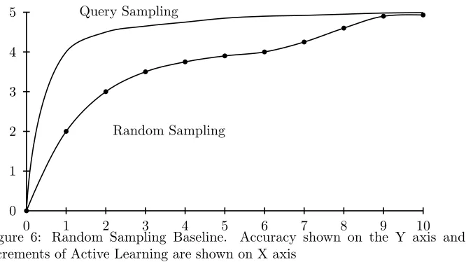
Figure 6: Random Sampling Baseline. Accuracy shown on the Y axis and increments of Active Learning are shown on X axis

However, random sampling is a very useful tool in examining the effectiveness of other methods. In short, an effective query selection technique should beat random sampling. For example in Figure 6 the area between the two curves shows the extra accuracy obtained by using active learning with some query selection algorithm versus using active learning with random sampling. In some of the literature this type of graph is shown with error rates instead of accuracy rates leading to the name “Banana graphs”.

3.6.2 Uncertainty Sampling

This method is very similar to that of boosting, where we direct the training of subsequent classifiers based on the misclassification of the current classifier. The main difference is that we do not know the true classification of the exam-ples in uncertainty sampling until we query the oracle. The stopping criterion for active learning is the number of examples the oracle is willing to classify. Ide-ally the most informative examples about the domain would be the unlabelled example about which the current classifier has the most difficulty in classifying. A probabilistic classifier is used in [LG94] to measure uncertainty, with those unlabelled examples which have a probability of0.5 being selected as queries. In the ideal case, for each iteration of active learning the number of queries n would be 1, but for efficiency reasonsncan be>1. In their experiments, unla-belled examples from above and below 0.5 are chosen, since there was evidence [HCOI91] showing that training on both sides of the decision boundary to be useful

The threshold used to decide when to classify an example based on its prob-ability estimate is given by the following equation.

l21P(C|w) +l22(1−P(C|w))> l11P(C|w) +l12(1−P(C|w))

wherel_ij is the cost associated with i being classified as j.

The experiments in [LG94] compared uncertainty sampling with random sampling and relevance sampling used on news story titles (AP newswire be-tween 1988 and early 1993). The choice of the initial classifier is important in this algorithm since there may be a low frequency class we are trying to con-struct a classifier for. Unless this initial classifier has some knowledge of this class a long period of random sampling may ensue until it happens to find an example of the desired class. In the experiments the initial classifier was sup-plied with three, randomly selected positive examples and the value of n used in each round of uncertainty sampling was 4. Relevance sampling was done by selecting the nexamples with the highest probability.

The result of the experiment was that uncertainty sampling performed better than the other two techniques (random sampling and relevance sampling) and performed comparably or better than a classifier trained on all the training data. Using uncertainty sampling and relevance sampling resulted in increased learning rates as compared with that of random sampling in the early stages of learning. Effectiveness levels achieved by 100,000 randomly chosen examples were achieved by uncertainty sampling using less than 1,000 examples.

Some drawbacks of the approach are that the final classifier produced was unstable. The authors believe this was caused by the randomness involved with selecting the three positive instance used for the initial classifier. When the three training data cases were not representative of the class being modelled, there was a considerable delay before uncertainty sampling found additional positive examples.

3.6.3 Query By Committee (QBC)

The Query By Committee algorithm [SOS92] [FSST97] fall under the category of stream based selection. The learner is given access to a stream of unlabelled examples drawn from the input space at random according to some unknown distribution D. As examples are drawn from the stream, the learner must decided whether reject the example (it can easily classify the example itself) or present the example to the oracle (it finds it difficult to classify the example).

Initially most examples will be informative for the learner since it has little knowledge of the target concept. As active learning continues, the prediction ca-pabilities of the learner will improve and it discards the majority of the examples drawn from the stream. Initially the learner will query the oracle extensively, this should subside reducing the workload for the oracle.

In [FSST97] the learner is given access to two oracles plus an algorithm.

Sample this oracle will return an example randomly selected from the domain according to some unknown distributionD

Label an oracle which will return the true label of the example supplied as the parameter.

Gibbs this computes the Gibbs prediction for an example using a randomly selected hypothesis from the current version space[Mit97].

In QBC the stopping criteria is measured on the number of rejection. A threshold is computed based on the prediction error and the desired reliability. While the stopping criteria are not met the following is done.

1. Sampleis called to get an instancex.

2. Gibbsis then called twice onx

3. If the two agree then the example is rejected (goto step 1)

4. Else Label is called to get the true classification of x. Update the ver-sion space to be the set of consistent hypothesis with the newly labelled instance.

As a brief example of stream based active learning, [NS04] shows an appli-cation for detecting and evaluating collisions at road junctions. The real world problem lends itself to stream based approach as it is linear in nature and the authors report good results when using stream based active learning.

3.6.4 Lookahead Algorithm

In [LMR99] a selective sampling methodology for the nearest neighbour classifier is presented. Most selective sampling methods focus on choosing examples from regions of uncertainty. The authors propose a method which will use a utility function for appraising classifiers and a posteriori class probability estimate for examples in the instance space (domain).

The method performance is comparable or better than random sampling, uncertainty sampling and maximal distance on both artificial and real world problems. Maximal distance is where the example selected is one which will have different labels amongst is three nearest neighbours and is the most distant from its closest labelled neighbour. Lookahead performs especially strongly when the instance space contains more than one region of some class, (e.g. two Gaussian). Lack of exploration in other methods results in failure to capture these in their models. The drawback with the lookahead method is its computational expense.

3.6.5 Bootstrap-LV

Presented in [STP04], Bootstrap-LV describes an active learning method for construction of class probability estimates (CPE). These are used to rank doc-uments in order of interest, or to present offers to users in order of probability of purchase (read, expected benefit to seller) rather than conduct a hard classi-fication.

The process first estimates the estimation variance (using the Local Vari-ance) of each example in the pool of unlabelled examples. If the LV is high, then the example is not well captured by the current model. The LV also cap-tures some information about the potential error reduction for other examples if the classification of this example were known. In Bootstrap-LV the LV estima-tions, together with a specialised sampling procedure, are used to identify the unlabelled examples that are particularly likely to reduce the average estimation error across the entire input space.

Bootstrap-LV deviates from the generic framework for a pool based sampling algorithm. It generates k bootstrap subsamples B_j for j = 1. . . k. It then induces a model E_j for each of the subsamples. These models are used to calculate the estimated variance for each example in the pool of unlabelled examples. The estimate (LV) is calculated by the variance amongst the Class Probability Estimations predicted by the models E_j. Finally each example in the pool of unlabelled examples is assigned an effectiveness score that is proportional to it LV.

The final part of the query selection function in Bootstrap-LV is selecting queries from the pool, this can be done in one of three ways. Direct selection

is where we select queries based on the effectiveness score of the unlabelled examples. Random selection can also be used. Weighted sampling is where we select unlabelled examples from the pool using a distribution where the probability of each example being sampled is proportional to its local variance. A serious limitation with this approach is that it incurs a large computation cost at each phase. The authors state that the method does become like random sampling after the initial phases, thus as an optimisation the authors suggest to only apply the method at the initial phases of active learning. Future work proposed includes applying the same weighted sampling technique with other metrics:

3.7

Related Work

There has been developments which do not change the query selection function, rather they alter the active learning framework. The addition of adaptive resam-pling techniques has seen some interest in the literature. In addition there has been work in the area of relevance feedback in the information retrieval arena, which is very similar to active learning in classification, except that instead of trying to optimise a classifier with respect to precision, the system should return the most relevant documents, thus recall also becomes important.

3.7.1 Active Learning using boosting and Bagging

In [AM98], Abe and Mamutsuka, propose a query learning strategy by com-bining the idea of QBC with boosting and bagging. This idea is also done by [STP04] in the bootstrap phase of Bootstrap-LV.Baggingworks by randomly resampling (with replacement) from the training data according to some (uni-form) distribution. For each of the subsamples produced, a classifier is induced from the subsample and the final classifier output is formed by a majority vote amongst the constituent classifiers. Boostingimproves the performance of a weak learner by repeatedly resampling the training data, with the distribution weighted each time in order to focus on misclassified examples. This can be done using a weighted sampling procedure. A common boosting technique is called AdaBoost [Sch99].

Query by Bagging, is where the at each stage of active learning, bagging is used to construct an ensemble of models from the set of labelled examples.

1. Resample according to a uniform distribution on the set of labelled exam-ples to create subsamexam-plesS1. . . ST

2. Induce a classifier using each subsample C1. . . CT

3. Find the instancexfor which there is maximal disagreement.

4. Obtain label for instancexand update the labelled set accordingly.

Query by Boosting is a slight adaption where the resampling distribution is changed in order to focus the next induced classifier C_t+1 on the examples

misclassified by C_t. The query selected is one for which the final hypothesis obtained by boosting has the least margin. The margin is the difference between the total weight assigned to the correct label and that assigned to the incorrect label.

1. Run AdaBoost on labelled examples to obtainhfin(x) =arg maxylog_βt1

2. Find the instancexfor which there is minimum margin x=arg min|_ht(x)=0log_βt1 −_ht(x)=1log_βt1|.

3. Obtain label for instancexand update the labelled set accordingly.

The termadaptive resampling refers to methods like boosting and bagging that adaptively resample data biased toward the misclassified examples in the training data, then combine the predictions of several classifiers. In [IAZ00] the authors apply adaptive resampling to active learning. The goal was to retain some of the advantages of adaptive resampling methods (e.g. accuracy and robustness of the generated model) and combine it with a reduction in the size of the required training set.

Active Learning using Adaptive Resampling (ALAR), presented in [IAZ00] uses two classification methods in each active learning phase. The first classifier (M1) is used to guess the labels of the unlabelled documents. A second classifier (M2) is induced from the labelled data set, using adaptive resampling to con-struct an ensemble of models. The next step selects a subset of examples from the unlabelled examples from the weights calculated using the guessed labels and the ensemble. These selected examples are then labelled by the teacher and added to the list of known labelled examples. For the final round of active learning the final classifier is the combination of the ensemble.

The resampling was done using the normalised version of the following weighting function for each instanceiin labelled examples.

w(i) = (1 +error(i)3)

where error(i) is the cumulative error for the instancei over all models in the ensemble.

In [AM98], Abe and Mamutsuka, propose a query learning strategy by com-bining the idea of QBC with boosting and bagging. This idea is also done by [STP04] in the bootstrap phase of Bootstrap-LV.Baggingworks by randomly resampling (with replacement) from the training dataset according to some (uni-form) distribution. For each of the subsamples produced, a classifier is induced from the subsample and the final classifier output is formed by a majority vote amongst the constituent classifiers. Boostingimproves the performance of a weak learner by repeatedly resampling the training dataset, with the distribu-tion weighted each time in order to focus on misclassified examples. This can be done using a weighted sampling procedure. A common boosting technique is called AdaBoost [Sch99].

Query by Bagging, is where at each stage of active learning, bagging is used to construct an ensemble of models from the set of labelled examples.

1. Resample according to a uniform distribution on the training dataset to create subsamplesS1. . . ST

2. Induce a classifier using each subsample C1. . . CT

3. Find the unlabelled examplexfor which there is maximal disagreement.

4. Obtain label forxand update the training dataset accordingly.

Query by Boosting is a slight adaptation where the resampling distribution is changed in order to focus the next induced classifier C_t+1 on the examples

1. Run AdaBoost on training dataset to obtainh_fin(x) =arg max_ylog_βt1

2. Find the unlabelled examplexfor which there is minimum margin x=arg min|_ht(x)=0log_βt1 −_ht(x)=1log_βt1|.

3. Obtain label forxand update the training dataset accordingly.

Whereβ_tcomes from AdaBoost andh_fin(x) is the final hypothesis produced by AdaBoost. In both cases, an improvement was seen when tried empirically. Query by Boosting showed more of an improvement than Query by Bagging. One point to mention is that both had a high time complexity which may impede use as an on-line method.

The termadaptive resampling refers to methods like boosting and bagging that adaptively resample data biased toward the misclassified examples in the training data, then combine the predictions of several classifiers. In [IAZ00] the authors apply adaptive resampling to active learning. The goal was to retain some of the advantages of adaptive resampling methods (e.g. accuracy and robustness of the generated model) and combine it with a reduction in the size of the required training dataset.

Active Learning using Adaptive Resampling (ALAR), presented in [IAZ00] uses two classification methods in each active learning phase. The first classifier (M1) is used to guess the labels of the unlabelled documents. A second classifier (M2) is induced from the training dataset, using adaptive resampling to con-struct an ensemble of models. The next step selects a subset of examples from the unlabelled examples from the weights calculated using the guessed labels and the ensemble. These selected examples are then presented to the teacher, labelled and added to the training dataset. The final classifier produced is an ensemble of the subsequent classifiers.

The resampling was done using the normalised version of the following weighting function for each instanceiin labelled examples.

w(i) = (1 +error(i)3)

where error(i) is the cumulative error for the instancei over all models in the ensemble.

3.7.2 Relevance Feedback

Relevance Feedback, as noted in [LG94], does a form of non-random sampling. After supplying a query, users are presented with a listing of instance which the current classifier finds most probable to belonging to the desired class. The user is asked to label these instances, normally as a relevant/not relevant label, with the feedback used to retrain the learner in order to return more relevant cases. This approach puts more onus on retrieval of relevant texts than production of a stable accurate final classifier with high precision. There is a claim [LG94] that relevance feedback has many problems as an approach to sampling. It works poorly as the classifier improves and is susceptible to selecting redundant examples.