A Supervised Approach for Sentiment Analysis using
Skipgrams
Javi Fernández, José M. Gómez, Patricio Martínez-Barco
Department of Software and Computing Systems
University of Alicante
{javifm,jmgomez,patricio}@dlsi.ua.es
Abstract
We present a supervised hybrid approach for Sentiment Analysis in Twitter. A sentiment lexicon is built from a dataset, where each tweet is labelled with its overall polarity. In this work, skipgrams are used as information units (in addition to words and n-grams) to enrich the sentiment lexicon with combinations of words that are not adjacent in the text. This lexicon is employed in conjunction with machine learning techniques to create a polarity classifier. The evaluation was carried out against different datasets in English and Spanish, showing an improvement with the usage of skipgrams.
1 Introduction
Twitter has become one of the most popular sources of data to extract subjective information from. Here, people share aspects and opinions about their everyday life. This subjective information has a great value for general users, but mainly for brands and organisations. They can monitor their reputation by analysing the sentiment of the tweets posted about them or their competitors. However, extracting this information accordingly in Twitter texts is a very challenging task for current Sentiment Analysis (SA) approaches. The short length of the tweets (140 characters), the
informality, and the lack of context, makes sentiment detection and extraction a far harder task. In addition, the vast amount of tweets (over 500 million tweets per day1) complicates traditional SA systems to process this subjective information in real time. The performance of SA tools has become increasingly critical.
In this paper we describe a sentiment analysis approach, that faces some of the challenges of analysing subjective information in Twitter, but taking into account its employment in real-time applications. The remainder of this paper is structured as follows. In Section 2 we briefly describe the related work in sentiment analysis and introduce our work. In Section 3 we detail the approach we propose. The evaluation performed and its discussion is provided in Section 4. Finally, Section 5 concludes the paper, and outlines the future work.
2 Related work
2.1 Sentiment Analysis
Sentiment Analysis
is the field of study that identifies and extracts subjective information from texts. Two main approaches can be followed: machine learning approaches and lexicon-based approaches [Taboada 2011, Medhat 2014].
Machine learning
approaches treat polarity classification as a text categorisation problem. Texts are usually represented as vectors of features, and depending on the features used the system can reach better results. If a labelled training set of documents is needed, the approach is defined as supervised learning; if not, it is defined as unsupervised learning. These approaches perform very well in the domain they are trained on, but their performance drops when the same classifier is used in a different domain [Pang 2008, Tan 2009]. In addition, if the number of features is big, the efficiency drops dramatically.Lexicon-based approaches make use of dictionaries of opinionated words and phrases to discern the polarity of a text. In these approaches, each word in the dictionary is assigned a score of positivity and negativity. To detect the polarity of a text, the scores of its words are combined, and the polarity with the greatest score is chosen. These dictionaries can be generated manually, semiautomatically from an initial seed of opinionated words [Kim 2004], or automatically from a labelled dataset [Cruz 2013]. The major disadvantage of the first one is the incapability to find opinion words with domain and context specific orientations, while the second one helps to solve this problem [Medhat 2014]. These approaches are usually faster than machine learning ones, as the combination of scores is normally a predefined mathematical function.
2.2 Skipgrams
Most of the current sentiment analysis approaches employ words, n-grams and phrases as information units for their models, either as features for machine learning approaches, or as dictionary entries in the lexicon-based approaches. However, words and n-grams have some problems to represent
the flexibility and sequentiality of human language. In the case of Twitter texts, a deeper analysis of the text is not possible or accurate because of the small size, lack of context (and sometimes lack of structure), and informality [Aranberri 2013]. In order to create n-grams that can represent the flexibility and sequentiality of human language, it is necessary to go further than just adjacent words. This is the reason why we decided to use of skipgrams in sentiment analysis.
The use of skipgrams is a technique whereby n-grams are formed (bigrams, trigrams, etc.), but in addition to using adjacent sequences of words, it also allows some words to be skipped [Guthrie 2006]. More generally, in a k-skip-n-gram, n determines the number of terms, and k the maximum number of skips allowed. In this way skipgrams are new terms that retain part of the sequentiality of the terms, but in a more flexible way than n-grams [Fernandez 2014]. Note that an n-gram can be defined as a 0-skip-n-gram, a skipgram where k=0. For example, the sentence “I love healthy food" has two word level trigrams: “I love healthy" and “love healthy food". However, there is one important trigram implied by the sentence that was not captured: “I love food". The use of skipgrams allows the word “health" be skipped, providing the mentioned trigram.
3 Methodology
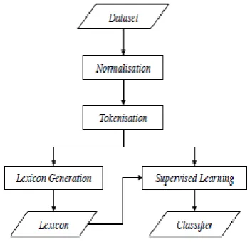
flow can be seen in Figure 1. In the following sections we describe this flow in detail.
Figure 1: System flow
3.1 Normalisation
As we do not want to lose the subjective information given by the original text, we perform a very simple normalisation. Employing a more complex normalisation can induce some errors that would be propagated to the final results. We start converting all the tweets to lower case. Usernames and URLs are replaced by the strings “USERNAME" and “URL" respectively, as they are not words that represent subjectivity. Hashtags were not modified as they can contain some information about the topic and sentiment about the tweets.
Then, we carry out a partial character repetition removal. If the same character is repeated more than 3 times, the rest of repetitions are removed. In this way, the words are normalised, but we can still recognise if the original words had repeated characters. We do not remove all repetitions as they can be very useful to detect subjectivity in texts [Saif 2012]. For example, the words “gooood" and “gooooood" would be normalised to “goood", but the word “good" would remain the same. We assume the ambiguity of this example, which can
refer to both “good" and “god". Figure 2 shows an example of this normalisation process.
So excited to go to #NewYork tomorrow with my best friend everrrrr @John!!!!
↓
so excited to go to #newyork tomorrow with my best friend everrrrr @john!!!!
↓
so excited to go to #newyork tomorrow with my best friend everrr @john!!!
↓
[image:3.614.97.273.107.277.2]so excited to go to #newyork tomorrow with my best friend everrr USERNAME!!! Figure 2: Example of normalisation process.
3.2 Tokenisation
Once we have normalised the texts, we extract all the terms they contain. We consider a term as a group of adjacent characters of the same type: groups of letters, groups of numbers or groups of punctuation symbols. For example, the text “want2go!!" would be tokenised to the terms “want", “2", “go", and “!!". These terms are extracted using regular expressions. Finally, we obtain the skipgrams by making the proper combinations of the terms extracted. Table 1 shows an example of this tokenisation process.
so excited to go to #newyork tomorrow with my best friend everrr USERNAME!!!
↓
(so) (excited) (to) (go) (to) (#) (HASHTAG) (with)
(my) (best) (friend) (everrr) (USERNAME) (!!!)
↓
(so excited) (so to) (excited to) (excited go) (to go) (to to) (go to) (go #) (to #) (to
(# newyork) (# tomorrow) (newyork tomorrow)
(newyork with) (tomorrow with) (tomorrow my)
(with my) (with best) (my best) (my friend) (best friend) (best everrr) (friend everrr) (friend USERNAME) (everrr USERNAME) (everrr !!!) (USERNAME) (USERNAME !!!)
Figure 3: Example of tokenisation process (skipgrams with n=2 and k=1)
3.3 Lexicon generation
Our sentiment lexicon consists on a list of skipgrams, where each skipgram has one value associated to different values of polarity, indicating how the term is related to that polarity. We called these values polarity scores. To build this lexicon, we need a polarity labelled dataset, which will provide both the skipgrams included in the dataset and their polarity scores. This scores depend on the number of the times the skipgram appears in text of a specific polarity, and the skips of the different occurrences. First, we explain some subscores, to understand the final formula:
• Skip score. This score penalises skipgrams with a high number of skipped terms. The formula applied is shown in Equation 1, where si
represents an occurrence of skipgram s in the dataset, and ks
i is the number of skipped terms of the occurrence si.
skip(si)= 1
ksi+1 (1)
• Polarity ratio score. This score indicates the proportion of texts of a specific polarity the skipgram appears in. It is calculated according the formula in Equation 2, where p
represents a polarity in the dataset, S is the set of occurrences of the skipgram s in the dataset, Sp is the set of occurrences of the skipgram s in texts labelled with polarity p. Note that this formula takes into account the skip score of the skipgram, in order to penalise skipgrams with a higher number of skipped terms.
(2) • Polarity confidence score. This score
boosts skipgrams that appear a high number of times in texts of a specific polarity. It is calculated as shown in Equation 3.
confidence(s,p)=1− | 1 Sp|+1
(3) The final polarity score for a specific skipgram is the product of its ratio score and its confidence score. The formula employed to calculate this score can be seen in Equation 4.
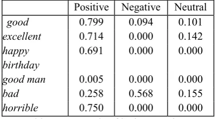
score(s,p)=ratio(s,p)⋅confidence(s,p) (4) At the end of this process we have a list of skipgrams with a score for each polarity: our sentiment lexicon. An example of entries2 in this lexicon can be seen in Table 1. As we can see in the example, positive words and expressions have a higher positive score, and negative words have a negative score. In addition, expressions like happy birthday or good man appear only in positive tweets, but happy birthday appears more times and than good man in the dataset, so its value is higher. Even the terms happy and birthday use to appear closer than the terms good and man, and this makes the difference much bigger.
Positive Negative Neutral
good 0.799 0.094 0.101
excellent 0.714 0.000 0.142 happy
birthday
0.691 0.000 0.000
good man 0.005 0.000 0.000
bad 0.258 0.568 0.155
horrible 0.750 0.000 0.000 Table 1: Example of lexicon entries.
3.4 Supervised learning
We use machine learning techniques to create a model able to classify the polarity of new tweets. The tweets in the dataset are employed as training instances, and the labelled polarities are used as categories. However, in contrast with text classification approaches, we employ the polarities also as features. The weight of each feature is calculated as specified in Equation 5, where weight(t,p) is the weight of polarity p in the text t, and St is the set of skipgrams in the text t.
(5) Table 2 shows an example of feature weighting for the text “I like football" using 1-skip-2-grams 3 . Each row represents a skipgram with a value for each polarity, calculated as score(s,p)⋅skips(si) . The
final row is the sum of all the previous values, which will be employed as feature weights for the machine learning process.
3 Obtained using the SemEval 2014 dataset
Positive Negative Neutral
I 0.422 0.220 0.356
like 0.354 0.406 0.235
football 0.346 0.540 0.102 I like 0.154 0.063 0.046 I football 0.046 0.037 0.017 like football 0.000 0.000 0.000
weight 1.322 1.266 0.756
Table 2: Example of features weights for the sentence “I like football" with
1-skip-2-grams
To build our model we employed Support Vector Machines (SVM), as it has been proved to be effective on text categorisation tasks and robust on large feature spaces [Sebastiani 2002, Mohammad 2013]. More specifically, we used the LibSVM [Chang 2011] default implementation (linear kernel, C=1, ε=0.1).
4 Evaluation
To obtain the results of our analysis we evaluated our approach against two datasets. Both of them are divided into a train dataset (to create the model) and a test dataset (to validate the model created). The distribution of these datasets is shown in Table 3.
• SemEval Dataset (2013-14). This dataset was created and employed for the Sentiment Analysis in Twitter task in the 2013 [Nakov 2013] and 2014 [Rosenthal 2014] editions of the SemEval4 workshop. It consists on 10,709 tweets in English at global level, with 3 categories: positive, negative and neutral. The neutral class covered both neutral and objective tweets. These tweets were manually annotated.
• TASS Dataset (2012-13). This dataset was created for the TASS5 workshop, specifically for the Sentiment Analysis task in the 2012 edition [Villena 2013]
[image:5.614.83.301.71.192.2]and the Sentiment Analysis at global level task in 2013 [Villena 2013B]. It contains 68,017 tweets in Spanish annotated at global level, with 6 categories: very positive, positive, neutral, negative, very negative and none. For our experiments we mapped these polarities into 3: positive, negative and neutral. The annotation process of these tweets was manual for the training dataset, but automatic for the test dataset, using a voting scheme from all the submissions participating in the competition.
SemEval TASS
Train Test Train Test
[image:6.614.328.521.272.438.2]Positive 2,510 1,572 2,783 22,233 Neutral 3,363 1,640 2,312 22,721 Negative 1,023 601 2,124 15,844 Total 6,896 3,813 7,219 60,798 Table 3: Datasets distribution in number of
tweets.
We chose these datasets because they are publicly available to the research community, they have been used several times in sentiment analysis competitions, and they are very different from each other, in terms of size, language, topic, and annotation process. For each dataset separately, a lexicon and a supervised model is generated using the train examples, and the model created is evaluated using the test examples.
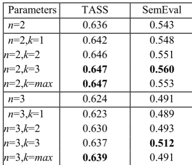
The results of our experiments are shown in Table 4. We do not use accuracy because it is not a good measure for text categorisation when using an imbalanced corpus Yang1999. Instead, we use the F1 (F-score with β=1) because it represents a balance between precision and recall of the measures of each polarity. Moreover, the F1 scores shown are the macro-average of all the F1 scores of the polarities, as it gives the same importance to
all polarities regardless of the number of examples in the dataset. The Parameters column refers to the n and k values employed for the k-skip-n-grams generation. However, for simplicity, the parameter n will represent the maximum number of terms allowed in a skipgram. For example, the experiments with n=3 will include skipgrams with n=3, n=2 and n=1. The notation n=max indicates there was no limit with the number of terms, and k=max indicates there was no restriction with the number of skips.
Parameters TASS SemEval
n=2 0.636 0.543
n=2,k=1 0.642 0.548
n=2,k=2 0.646 0.551
n=2,k=3 0.647 0.560
n=2,k=max 0.647 0.553
n=3 0.624 0.491
n=3,k=1 0.623 0.489
n=3,k=2 0.630 0.493
n=3,k=3 0.637 0.512
[image:6.614.86.303.288.390.2]n=3,k=max 0.639 0.491 Table 4: Results of the evaluation (F1 score)
appear together in some cases and the skipgram modelling has discovered, useful to determine the polarity of a text. Even tough the size, topic, language, and annotation process of these datasets is very different, the evaluation shows a robust improvement with the usage of skipgrams in both datasets.
5 Conclusions
In this paper we presented a supervised hybrid approach for Sentiment Analysis in Twitter. We built a sentiment lexicon from a polarity dataset using statistical measures. We employed skipgrams as information units, to enrich the sentiment lexicon with combinations of words that do not appear explicitly in the text. The lexicon created was used in conjunction with machine learning techniques to create a polarity classifier.
The evaluation was carried out against very different datasets, in terms of size, topic, language, and annotation process, and showed an improvement with the usage of skipgrams in all datasets. More specifically, just increasing the maximum allowed number of gaps between the words in the skipgrams (k), the results obtained were up to a 3.1% better. This suggested that there are some sentiment-specific combinations of words discovered by the skipgram modelling, that do not appear explicitly together.
As future work, we plan to study new methods to calculate and combine the weight of the skipgrams. In addition, we want to include external resources and tools, such as a more complex normalisation, or knowledge from existing sentiment lexicons like SentiWordNet. We will also extend our study to different corpora and domains, to confirm the robustness of the approach.
Acknowledgments
This research work has been partially funded by the Spanish Government and the European Commission through the project, ATTOS (TIN2012-38536-C03- 03), LEGOLANG (TIN2012-31224), SAM (FP7- 611312) and FIRST (FP7-287607).
References
Nora Aranberri, Pablo Gamallo, and Lluis Padr. 2013.Introduccion a la tarea compartida Tweet-Norm 2013: normalización léxica de tuits en español. In XXIX Congreso de la Sociedad Española de Procesamiento de Lenguaje Natural (SEPLN 2013).
Chih-chung Chang and Chih-jen Lin. 2011. LIBSVM: A Library for Support Vector Machines. ACM Transactions on Intelligent Systems and Technology (TIST), 2:1–39.
Ferm´ın L Cruz, Jose A Troyano, Fernando Enríquez, F Javier Ortega, and Carlos G Vallejo. 2013. Long autonomy or long delay? the importance of domain in opinion mining. Expert Systems with Applications, 40(8):3174–3184.
Javi Fernández, Yoan Gutiérrez, José M. Gómez, and
Patricio Martínez-Barco. 2014. GPLSI:
Supervised Sentiment Analysis in Twitter using Skipgrams. In Proceedings of the 8th International Workshop on Semantic Evaluation (SemEval 2014), number SemEval, pages 294–299.
David Guthrie, Ben Allison, Wei Liu, Louise Guthrie, and Yorick Wilks. 2006. A Closer Look at Skip- gram Modelling. In 5th international Conference on Language Resources and Evaluation (LREC 2006), pages 1–4.
Soo-min Kim, Marina Rey, and Eduard Hovy. 2004. Determining the Sentiment of Opinions. In Proceedings of the 20th International
Conference on Computational Linguistics
Walaa Medhat, Ahmed Hassan, and Hoda Korashy. 2014. Sentiment Analysis Algorithms and Applications: a Survey. Ain Shams Engineering Journal.
Saif M. Mohammad, Svetlana Kiritchenko, and Xiao- dan Zhu. 2013. NRC-Canada: Building the State- of-the-Art in Sentiment Analysis of Tweets. In Proceedings of the International
Workshop on Semantic Evaluation
(SemEval-2013).
Preslav Nakov, Sara Rosenthal, Alan Ritter, and Theresa Wilson. 2013. SemEval-2013 Task 2: Sentiment Analysis in Twitter. In Proceedings of the International Workshop on Semantic Evaluation (SemEval-2013), volume 2, pages 312–320.
Bo Pang and Lillian Lee. 2008. Opinion Mining and Sentiment Analysis. Foundations and Trends in Information Retrieval, 2(1–2):1–135.
Sara Rosenthal and Alan Ritter. 2014. SemEval-2014 Task 9 : Sentiment Analysis in Twitter. In Proceedings of the 8th International Workshop on Semantic Evaluation (SemEval 2014), pages 73–80.
Hassan Saif, Yulan He, and Harith Alani. 2012. Sentiment Analysis of Twitter. In Proceedings of the 11th International Semantic Web Conference (ISWC 2012), pages 11–15.
Fabrizio Sebastiani. 2002. Machine Learning in Automated Text Categorization. ACM Computing Surveys (CSUR), 34(1):1–47, March.
Maite Taboada, Julian Brooke, Milan Tofiloski, Kimberly Voll, and Manfred Stede. 2011. Lexicon- based methods for sentiment analysis. Computational Linguistics, 37(2):267–307.
Songbo Tan, Xueqi Cheng, Yuefen Wang, and Hongbo Xu. 2009. Adapting Naive Bayes to Domain Adaptation for Sentiment Analysis. Advances in Information Retrieval, pages 337–349.
Julio Villena-Roma´n and Janine Garcıa-Morera. 2013. TASS 2013-Workshop on Sentiment Analysis at SE- PLN 2013: An overview. In XXIX Congreso de la Sociedad Española de Procesamiento de Lenguaje Natural (SEPLN 2013).
Julio Villena-Roman, Eugenio Martınez-Camara,
Sara Lana-Serrano, and Jose Carlos
Gonzalez-Cristobal. 2013. TASS - Workshop
on Sentiment Analysis at SEPLN.
Procesamiento del Lenguaje Natural, 50:37–44.