Predicting Probability Distributions for Surf Height Using an Ensemble of Mixture Density Networks

Predicting Probability Distributions for Surf

Height Using an Ensemble of Mixture Density

Networks

Michael Carney, P´adraig Cunningham, Jim Dowling and Ciaran Lee

Trinity College Dublin

Abstract. There is a range of potential applications of Machine Learn-ing where it would be more useful to predict the probability distribution for a variable rather than simply the most likely value for that vari-able. In meteorology and in finance it is often important to know the probability of a variable falling within (or outside) different ranges. In this paper we consider the prediction of surf height with the objective of predicting if it will fall within a given ‘surfable’ range. Prediction prob-lems such as this are considerably more difficult if the distribution of the phenomenon is significantly different from a normal distribution. This is the case with the surf data we have studied. To address this we use an ensemble of mixture density networks to predict the probability den-sity function. Our evaluation shows that this is an effective solution. We also describe a web-based application that presents these predictions in a usable manner.

1

Introduction

There are many prediction problems where simple ‘point’ predictions are not adequate to guide action. In meteorology and in finance it is often important to know the probability of a variable falling within (or outside) different ranges. It might be that a 20% probability of flooding may be enough to place emergency services on alert. Or the best returns in financial trading might come from events that have a small but significant probability. Problems such as these have gen-erated an interest in the area of probability density forecasting. Research in this area is complicated because the data may have a multi-modal generating distri-bution. In addition, in many scenarios, variance is input-dependent. Recently, research in the financial domain has suggested that the reason why non-linear models do not perform significantly better than linear models is because the non-linearity in the data is due to input-dependent higher order moments (Clements & Smith, 2000).

density function. The surf data has a highly skewed unconditional distribution. We intend to show that our ensemble of probabilistic models can outperform standard neural networks on data that is conditionally skewed. We use Mixture Density Networks (MDNs) as our base model, this class of model has been shown to be successful for complex multi-valued functions where standard regression models fail.

The paper is laid out as follows. In Section 2 the details of the surf prediction problem are presented. In Section 3 a review of the issues associated with pre-dicting distributions is presented and our method based on ensembles of Mixture Density Networks is described. Section 4 discusses the issues posed in evaluating density predictions and describes the metrics we use. These metrics are used to analyze the performance of the ensemble of MDNs on artificial data in Section 5. The Surf Prediction Engine is described in Section 6 and an evaluation of its performance is presented in Section 7.

2

The Surf Prediction Problem

The popular sport of surfing requires suitable ocean and weather conditions. Of specific interest to surfers is the near-shore wave height at locations where surf breaks are accessible. The prediction of wave heights is aided by the US National Oceanic and Atmospheric Administration (NOAA) which provides open ocean wave forecasts online for specific locations in the Pacific and Atlantic oceans (Tolman, 1999). Any ocean wave can be characterised as a vector quantity, with the direction expressed in terms of degrees (clockwise, from Polar North) and the magnitude represented by two scalar quantities: the wave height (vertical distance from trough to crest) and its period (Komen et al., 1994). The period of a wave is directly proportional to its kinetic energy. NOAA generates forecasts of ocean waves using both the WAM model (Hasselmann et al., 1988), a model of the physical processes governing wave evolution, and real-time data from moored buoys. Seven-day forecasts are provided for the estimated height, period and direction of waves at the buoy locations. The relationship, however, between open ocean wave height and the subsequent surf height at near-shore surf breaks is complex. Physics allows us to model how waves can be refracted, reflected, diffracted and ultimately break when they come into contact with shallow water or land (Butt et al., 2004). However, mathematical models based on physics require precise parameters not only of the wave dynamics at buoys, but also of islands, shoreline features, the angle of exposure of the surf break and the profile of the sea floor around the surf break. Partial, informal information on these parameters is available in surf guides (Colas, 2004) (e.g. minimum and maximum height at which waves are surfable), but due to the lack of available information on the many other parameters, it is not currently possible to build general linear or non-linear models for predicting wave heights at the diverse surf breaks around the world.

well calibrated mixture density networks to obtain accurate forecasts of the prob-able maximum surf-zone wave heights given data buoy readings. The ensemble is trained on data that combines the environmental readings from the off-shore data buoy with local, expert, visual recordings of the surf-zone maximum wave heights.

We have compiled a new database that combines surf zone observations with off-shore buoy readings. The data used in this study comes from two primary sources. The off-shore environmental data needed to make the near-shore surf predictions comes from a moored buoy1 _{off the south west of Ireland. The}

ob-servations of the near-shore wave heights are recorded by a surf expert2_{. The}

observations are coupled with the buoy data by calculating the time delay be-tween the buoy reading and the experts observation using the wave period and buoy to shore distance. The database contains 260 vectors.

3

Predicting Distributions

The standard solution to regression problems is to apply a sum-of-squares error function to N training data pairs, (x1, t1), ...,(xn, tn), to predict a conditional mean of a new unseen data vector,htn+1|xn+1i. This form ofpoint prediction is

often inadequate in practice because there is no indication of the level of uncer-tainty in the model’s predictions. The most rudimentary method of quantifying this uncertainty is to report a mean-squared-error (MSE). This is the average uncertainty in the model over the complete input training set. The combination of a point prediction with MSE makes the assumption that the uncertainty in the model is described by a Gaussian conditional density function with constant variance equal to the MSE.

Quantifying the uncertainty in each individual prediction is our goal. To model this uncertainty we could use confidence intervals, however, De Finetti (1974) argues that the only concept needed to express uncertainty is probability, and so all predictions over a future event should be made in terms of probability distributions. Consequently, our goal, and the goal when making any prediction with uncertainty, is to create a model of the process as a sequence of probability density functions. This means that for any given input value e.g.xn+1, our model

should produce a conditional density functionp(tn+1|xn+1).

There exist a number of approaches to obtain estimates of the conditional density function. Fraser and Dimitriadis (1993) initially developed a Hidden Fil-ter Hidden Markov Model using the EM algorithm to produce predictions of conditional density forecasts. Weigend and Nix (1994) suggest a neural network architecture that predicts the mean value and the local error bars (standard de-viations) for given inputs, however, this approach assumes the data generating

1

The National Center for Environmental Prediction (NCEP) maintains a num-ber of buoys in the eastern Atlantic, our data comes from buoy 62081. See http://www.ncep.noaa.gov/

2

distribution is a Gaussian. Neuneier et al. (1994) and Bishop (1995) developed a semi-parametric conditional density estimation network or mixture density net-work (MDN)3_{. This approach removes the need to assume a Gaussian and can}

model unknown distributional shapes. Husmeier (1999) developed a two hid-den layer universal approximator called a random vector functional link (RVFL) which also can predict the whole conditional density function. Husmeier com-pares his RVFL model with an MDN and shows that both techniques produce results with equivalent accuracy. In this paper we will use an ensemble of MDNs to make stable, accurate predictions of conditional density functions.

There are two important points that restrict predicting the true generating distribution. Firstly, to define the true conditional density function accurately infinite parameters may be required. Secondly, each prediction is afunction, not a value; however, this function is estimated from observations alone. The aim of a probabilistic model is to simulate the real conditional density function as accurately as possible.

3.1 Ensembles of Mixture Density Networks

Mixture Density Networks (MDN) refer to a special type of ANN in which the target is represented as a probability distribution, or, more specifically, a con-ditional probability density function. MDNs were first introduced by Bishop (1995) and shown to successfully describe the conditional distribution for the multimodal, inverse problem and Brownian process. Since then they have been successfully applied to both financial (Schittenkopf et al., 2000) and meteorolog-ical data sets (Cornford et al., 1999).

MDNs represent the conditional density function by a weighted mixture of Gaussians known as a Gaussian Mixture Model(GMM). GMMs are a flexible, convenient, semi-parametric means of modeling unknown distributional shapes. The conditional density function is described in the form

p(t|x) = C

X

i=1

αi(φi(t|x)) (1)

whereφi is a Gaussian as follows,

φi(t|x) = 1 (2π)q/2_σ

i(x)c

exp(−kt−µi(x)k 2

2σi(x)2

) (2)

whereC is the number of components in the mixture. The parameterαi is the Gaussian weight or mixing coefficient andφi(t|x) represents theith Gaussian component’s contribution to the conditional density of the target vectort. For a full discussion on the Mixture Density Network architecture see (Bishop, 1995).

3

Due to the complexity of the local error curvature, straightforward gradi-ent descgradi-ent fails to optimise MDNs. To overcome this problem the optimisation technique requires dynamic adjustment of the learning rate during the training process to efficiently converge to a global minimum. We use Scaled Conjugate Gradients (SCG)(Moller, 1993) for optimisation of our Mixture Density Net-works. SCG uses the second derivative Hessian matrix to find the most direct route to the minimum.

With any neural network optimisation there is an inherent instability. This is due to the random initialisation of the network’s weight vectors. One approach to reducing the instability in a neural network is to train several neural networks and return an aggregate prediction. This is called the ensemble technique. There are two primary requirements for any ensemble approach,diversity in the indi-vidual networks, and the ability to aggregate your results. Two approaches to achieving these requirements are Bagging (Breiman, 1996) and Boosting (Freund & Schapire, 1996). We have implemented both and outline our implementations below.

3.2 Bagging MDNs

Bagging is an abbreviation for bootstrap aggregation. It uses the bootstrap, a statistical re-sampling technique, to generate multiple, diverse, training sets for networks of an ensemble. A bagged neural network ensemble generates training data for each ensemble member by sampling from the bootstrap empirical dis-tribution. A training set is created for each neural network in the ensemble and the networks are trained on this data.

Sporadically MDNs do not converge to a good solution due to a very poor random starting position. To reduce the effect of these weak solutions on the ensemble prediction we integrate the member solutions using a form of balancing (Heskes, 1997). The training sets in a bagged ensemble are generated by sampling with replacement from the original training set T. The probability that the individual training vector, taken from T, will not be part of a bootstrap re-sampled training set,Tbootstrap_{, is (1−1/N)}N_{≈0.368 whereN is the number} of training vectors in T. These omitted training vectors make a new out-of-bootstrap (oob) test set,Tobb _{for the ensemble member trained withT}bootstrap_. For each ensemble member we calculate the error, Eoob_{, over the vectors in its}

Toob_{. We use these error values to weight each member’s contribution to the} ensemble prediction. Assuming there areM ensemble members,

p(t|x) = M

X

i=1

C

X

j=1

Eoob i αi,j

PM

k=1Ekoob

(x)φi,j(t|x) (3)

3.3 Boosting MDNs

We have implemented AdaBoost.R2 (Drucker, 1997) for MDNs. The means of obtaining diverse training sets is distinctly different in boosting to bagging. In boosting, training of ensemble members is carried out sequentially. The vectors that have been ‘difficult’ for ensemble members to estimate i.e. obtain large errors, are more likely to appear in the training sets of subsequent ensemble members. This restricts ensemble members from being trained in parallel, how-ever, it has the advantage of reducing the bias of the resulting ensemble.

To combine the ensemble members a weighted median approach is used, the better performing members are assigned a heavier weighting. Integration is achieved in a similar way to the balancing method above; however, instead of using out-of-bootstrap vectors alone the whole training set is used to calculate the weightings.

4

Evaluating Probability Forecasts

A significant problem with probabilistic forecasting models is determining a means of evaluating the results. If we assign some probability to the actual observation, can the prediction be wrong? To determine whether a probabilistic model performs well you must first decide on your goals. The objective when making a density forecasting model is to, 1) create probability density func-tions that accurately predict the region in which the target lies and, 2) provide well calibrated probability estimates (Gneiting & Raftery, 2004). The first crite-rion refers to the spread of the predictive density about the target. The second criterion, calibration, is a measure of the statistical consistency between the dis-tributional forecasts and the observations. For example, a well calibrated model over 100 predictions for 100 events giving a particular outcome a 10% probability would result in that outcome occurring 10 times.

In this paper we use three error scores. Firstly, we use the average negative log predictive density (NLPD) (Good, 1952). This is the average value of the negative of the logarithm of the predictive densityp(...) at each observationt.

N LP D= 1

N

N

X

i=1

−log(p(yi|xi)) (4)

The third error score we use is the most comprehensive, the Continuous Ranked Probability Score or the CRPS. The CRPS (Gneiting & Raftery, 2004), is a generalisation of the Brier Score. The advantage of this error score is that it takes the whole distribution into consideration when measuring the error. The CRPS score uses the cumulative probability density function to determine the error.

crps(p, t) =−

∞

Z

−∞

(p(y|x)−H(y, t))2

dy (5)

whereH(x, t) is the Heaviside function i.e.

H(x, t) =1{x≥t} (6)

This function has a value of 1 ifx is greater thant, otherwise it has a value of 0. This is a strictly proper scoring rule, i.e. the forecaster will maximise their result for the forecastF if they use the forecastF, rather than anyG6=F. This is our preferred metric for scoring error because of its sensitivity to distance. We use the averagecrpsto evaluate the results of a complete input set.

CRP S= 1

N

N

X

i=1

crps(pi, yi) (7)

5

Analysis of Ensembles of MDNs on Artificial Data

−0.2 0 0.2 0.4 0

50 100

(b) ENN Errors

−0.2 0 0.2 0.4 0

50 100

(c) ε − Noise

0 0.5 1 1.5 2 −1.5 −1 −0.5 0 0.5 1 (d) EMDN

0 0.5 1 1.5 2 −1.5 −1 −0.5 0 0.5 1

(a) ENN with MSE

p(t|x) t(x) = f(x) + ε(x) f(x)

p(t|x) t(x) = f(x) + ε(x)

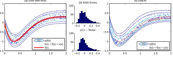
To demonstrate the MDNs ability to produce estimates of the higher moment conditional density effects we created a simple synthetic data set. Inputs for the data are uniformly drawn from the interval [0,2]. The target values are generated according to

t(x) = 4.26(e−x

−4e−2x_{+ 3e}x_{) +ǫ(x). (8)}

where ǫ(x) represents random sample noise drawn from the following distribu-tion,

SN(x) = 2 0.2φ(

y+ 0.1 0.2 )Φ(λ

y+ 0.1

0.2 ) (9)

SN is the skew normal function (Azzalini, 1985) that produces skewed distribu-tions.φ(x) is the probability density function andΦ(x) is the cumulative density function.λis the shape or skew parameter, a positive value results in a positive skew and vice versa. Whenλis 0 the distribution is symmetric.

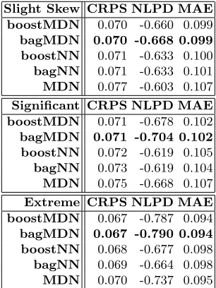
We generated 400 data pairs for training and 400 for testing. The test set is illustrated in Figure 1. For our experiment we trained five different types of networks; two ensembled point predictors, one trained with boosting (boostNN), the other bagging (bagNN); two ensembled MDNs, again one boosted (boost-MDN) and one bagged (bag(boost-MDN), and a single MDN. The single MDN and the MDN ensemble members have a 2 Gaussian GMM output. We carried out tests for three different values of λ(3 - slight skew, 6 - significant skew, 9 - extreme skew). The variance is constant so that we can measure the effects of the skew.

Table 1.Experiment results for synthetic data

Table 1 shows the average result over 10 runs for the three different exper-iments. The ensembles of MDNs provide the best predictions over all datasets. The single MDNs instability problem is also observed as the MDN performs poorly on the slightly skewed data but comparatively better on the more skewed data.

6

The Surf Prediction Engine

The surf prediction data is an example of a data set which has an underlying noise dynamic that shows evidence of higher moment influence. To demonstrate this we carried out the following experiment. We used 10-fold cross-validation with a standard bagged ensemble of neural networks and calculated the skew of the out-of-sample errors over all folds. The skew of this distribution is 2.25 for the surf data4_{. This is a significant skew compared to a normal distribution.}

Standard noise caused by observation errors would naturally assume a Gaussian shape. If we assume that ensembles of standard neural networks are a good means of obtaining well generalised predictions and we observe that the residuals of the results from the ensemble of neural networks have significant higher moment influences, we can conclude that these higher moment influences are present as an underlying dynamic in the data. This is the case in the analysis on artifi-cial data presented in Figure 1. The skew of the residuals is almost identical to the skew of the added noise. Now that we have determined the surf data is affected by skewness we can continue to develop a prediction engine that takes this information into consideration.

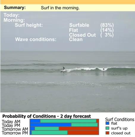
The boosted MDN is the base model for our surf prediction engine (see Figure 2). It is trained on the database described in Section 2 and produces conditional density forecasts for future events. Once a conditional density forecast has been made, this information can be used by the surfer. The most useful means of extracting the required information from the model is for the surfer to specify the wave heights that they can surf i.e. their ‘surfable’ range and the times in which they would like to surf. The engine will then determine from the predicted conditional density function the probability of those conditions. In this sense the model is giving a prediction that is tailored to the user. By providing this auxiliary information the decision maker can make a more informed choice.

7

Performance Evaluation

Figure 1 (a) shows 10 probability distributions derived from the predicted con-ditional density functions of the boosted ensemble of MDNs. This type of pre-diction gives the user a number of useful pieces of information. Firstly, between zero and four feet there is little uncertainty for these predictions. However, the model is much more uncertain about predictions of days when the actual surf height is higher. The tenth prediction is for the largest target and the probability

4

Fig. 2.This is a demonstration of the surf prediction engine forecasting waves in the range 3 - 6ft. with 83% probability. Detailed predictions for the morning are given at the top with an image of the most similar day shown. A two day summary chart is given at the bottom that shows the probability of the different classes. Predictions are provided over a seven day horizon.

distribution shows a large amount of uncertainty (broad distribution). Figure 1 (b) plots the position of the median and mode values of the predicted distribu-tions. The mode is the highest point on the distribution and represents the most typical outcome. The median is the point that divides the distribution in half. The plot shows that the model’s predicted median and mode are a good point estimate of the observed values.

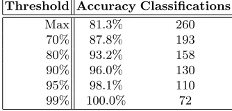
1 (b) confirms that the ensemble of MDNs is a useful predictor in the classic point estimate sense. However, we need to evaluate the accuracy in terms of the ‘surfable range’ predictions as presented to the user in Figure 2. Intuitively, an acceptable model from a users perspective is one that is correct on average 83% of the time on predictions that have an 83% confidence. For our model this is the case, as shown in Table 2. In this scenario the surfer has specified a 3ft - 6ft surfable range and predictions have been produced for 260 test days5_.

We can see from the table that the error is well correlated with the prediction

5

0 5 10

1 2 3 4 5 6 7 8 9 10

Surf Height (ft)

EMDN − Conditional Probability Density Function predictions

0 5 10

1 2 3 4 5 6 7 8 9 10

Surf Height (ft)

EMDN − Median Mode predictions

targets median prediction mode prediction

Fig. 3.(a) 10 out-of-sample predictions from a boostMDN on the surf data. The hor-izontal lines through each distribution represent the target observations. (b) shows the median and mode predictions relative to the target observations of the predicted density functions.

confidence. The results show that the boosted ensemble of MDNs has a slightly over-cautious bias, but in general is well calibrated and consistent. The number of correct predictions with respect to incorrect predictions obeys the thresholds assigned i.e. when the threshold is set to 95% then the model is correct≥95% of the time.

Table 2. boostMDN results for prediction of surfable range 3 - 6 ft. The accuracy column represents the percentage of correct predictions given the threshold. The Clas-sifications column represents the number of instances where the probability for a class exceeded the threshold.

Threshold Accuracy Classifications

Max 81.3% 260

70% 87.8% 193

80% 93.2% 158

90% 96.0% 130

95% 98.1% 110

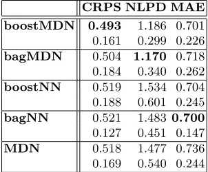
Finally, we evaluate the ensemble of MDNs predictions on the surf data against our benchmark models, the ensembles of NNs and a single MDN. These results are shown in Table 3 with the best score on each metric highlighted in bold. These figures are based on a 10-fold cross validation and the variances over the 10-folds are also shown underneath each error score. The boostMDN and bagMDN perform best on the probabilistic error measures; however, they also perform comparably to the ensembles of NNs on the MAE score.

Table 3.Results of experiments with surf data

CRPS NLPD MAE boostMDN 0.493 1.186 0.701 0.161 0.299 0.226 bagMDN 0.504 1.170 0.718 0.184 0.340 0.262 boostNN 0.519 1.534 0.704 0.188 0.601 0.245 bagNN 0.521 1.483 0.700 0.127 0.451 0.147 MDN 0.518 1.477 0.736 0.169 0.540 0.244

8

Conclusions

There are a range of applications for Machine Learning where a simple point prediction is not adequate to guide decision making, for instance in meteorol-ogy and finance. In this paper we present such an application. Surf prediction involves forecasting whether conditions on a surfing beach will be suitable for an individual given their acceptable range of wave heights. We use an ensemble of MDNs to predict the probability distribution for the maximum wave height. The application uses this distribution to estimate the probability that the surf height will be within the range desired by the user.

Bibliography

Azzalini, A. (1985). A class of distributions which includes the normal ones. J. Statist.(pp. 171–178).

Bishop, C. M. (1995).Neural networks for pattern recognition. Oxford University Press, Inc.

Breiman, L. (1996). Bagging predictors. Machine Learning(pp. 123–140). Butt, T., Russell, P., & Grigg, R. (2004). Surf science: An introduction to waves

for surfing. Alison Hodge.

Clements, M. P., & Smith, J. (2000). Evaluating the forecast densities of linear and non-linear models: Applications to output growth and unemployment.

Journal of Forecasting. Chichester.

Colas, A. (2004). The world stormrider guide. Low Pressure Publishing. Cornford, D., Nabney, I. T., & Bishop, C. M. (1999). Neural network-based

wind vector retrieval from satellite scatterometer data. Neural Computing and Applications.

De Finetti, B. (1974). Theory of probability, volume 1. Wiley.

Drucker, H. (1997). Improving regressors using boosting techniques. ICML(pp. 107–115).

Fraser, A. M., & Dimitriadis, A. (1993). Forecasting probability densities by using hidden markov models with mixed states. Time Series Prediction: Fore-casting the Future and Understanding the Past. Addison Wesley.

Freund, Y., & Schapire, R. E. (1996). Experiments with a new boosting algo-rithm. ICML (pp. 148–156).

Gneiting, T., & Raftery, A. (2004). Strictly proper scoring rules, prediction, and estimation(Technical Report 463). University of Washington.

Good, I. J. (1952). Rational decisions. Journal of the Royal Statistical Society. Series B (Methodological).

Hasselmann, S., Hasselmann, K., Bauer, E., Janssen, P., Komen, G., Bertotti, L., Lionello, P., Guillaume, A., Cardone, V., Greenwood, J., Reistad, M., Zam-bresky, L., & Ewing, J. (1988). The wam model-a third generation ocean wave prediction model. Journal of Physical Oceanography(pp. 1775–1810). Heskes, T. (1997). Balancing between bagging and bumping.Advances in Neural

Information Processing Systems(pp. 466–472).

Husmeier, D. (1999). Neural networks for conditional probability estimation: Forecasting beyond point predictions. Springer.

Komen, G., Cavaleri, L., Donelan, M., Hasselmann, K., Hasselmann, S., & Janssen, P. (1994). Dynamics and modelling of ocean waves. Cambridge University Press.

Moller, M. (1993). A scaled conjugate gradient algorithm for fast supervised learning. Neural Networks(pp. 525–533).

Schittenkopf, C., Dorffner, G., & Dockner, E. J. (2000). Forecasting time-dependent conditional densities: A semi-nonparametric neural network ap-proach. Journal of Forecasting. Chichester.

Tolman, H. (1999). User manual and system documentation of wavewatch-iii version 1.18. NOAA, Technical Note 166(p. 110).