Dynamic Evaluation Design

Munich Personal RePEc Archive

Dynamic Evaluation Design

Smolin, Alex

University of Bonn

October 2017

Dynamic Evaluation Design

∗

Alex Smolin

October 12, 2017

Abstract

A principal owns a firm, hires an agent of uncertain productivity, and designs a dy-namic policy for evaluating his performance. The agent observes ongoing evaluations and decides when to quit. While not quitting, the agent is paid a wage proportional to his perceived productivity; the principal claims the residual performance. After quit-ting, the agent secures a fixed safe payoff. I show that equilibrium evaluation policies are Pareto efficient and leave no rents to the agent. In a minimally informative equilib-rium, for a broad class of performance technologies, the agent’s wage deterministically grows with tenure.

Keywords: evaluation, information design, career concerns, bandit

experimenta-tion, downward wage rigidity, up-or-out

JEL Codes: C72, D82, D83, M52

1

Introduction

Evaluation of individual performance is an important part of organizational life. Although much evaluation is informal, most organizations have formal evaluation policies designed to collect and distribute performance information to employees.1 _{As communication and} information technologies advance, many companies find it easier to provide more evalua-tion. As a recent example, in August 2015 General Electric (GE) announced an ongoing shift from its legacy system of annual performance reviews to more frequent conversations between managers and employees via an online application.2 _{This way, GE joined other} high-profile companies such as Microsoft, Accenture, and Adobe in a move towards more frequent, exhaustive, and real-time evaluation. However, whenever adopting new evaluation policies the companies should ask: What is their effect on the overall performance? Would other evaluation policies do better? Ultimately, which evaluation policy is the best for the company?

In this paper, I develop a framework to analyze the design of evaluation policies. I consider a principal who owns a firm and hires an agent to work over time. The agent’s productivity, his type, is initially uncertain to both players but affects the agent’s ongoing performance. The performance is not directly observed but can be revealed through evaluations. While at firm, the agent is paid a wage proportional to his expected productivity; the principal claims the residual performance. In every period, the agent evaluates his career prospects and decides whether to quit. If the agent quits, he stops performing and secures an exogenously fixed safe payoff. Both players are risk neutral and discount the future at the same rate.

The principal designs and adopts a dynamic evaluation policy. The policy is a sequence of statistical experiments informative about past performance. The experiments can vary in what and when performance is assessed. The evaluation is costless but its design should take into account the agent’s incentives. On one hand, the promise of future evaluations motivates the agent to stay at the firm and learn whether he is able to perform well. On the other hand, any evaluation may turn out negative and persuade the agent to quit. As a result, a partially informative policy can outperform both no-evaluation and complete-evaluation policies. I discuss it in detail in the Section 3 example.

In Section 4, I investigate equilibrium evaluation policies by developing an efficiency argument. First, I show that the design problem can be viewed as a dynamic persuasion problem in a bandit experimentation setting. Doing so simplifies the problem and allows me

1_{According toMurphy and Cleveland(1995), between 74% and 89% of business organizations had formal}

performance appraisal policies by 1995.

2_{“GE’s Real-Time Performance Development,” Harvard Business Review, August 12, 2015,}

to characterize the set of feasible payoffs that can be possibly achieved in the relationship. Second, I study the set of implementable payoffs, achievable by some evaluation policy and the agent’s best response to it. I show this set includes all Pareto efficient payoffs that deliver the agent at least his safe option. I conclude that any equilibrium evaluation policy is efficient and leaves the agent with no rents. Furthermore, I characterize a minimally informative equilibrium policy. This policy turns out to be simple—it informs the agent whether he would quit if he could fully observe past performance but valued his outside option less.

In Section 5, I study effects of optimal evaluation on the agent’s career and wage dy-namics. I observe several qualitative properties that hold in the minimally informative equi-librium. First, the agent’s wage is a deterministic function of tenure. Second, for a broad class of performance technologies, the agent’s wage monotonically increases with tenure. The increase reflects the ongoing positive selection and the corresponding growth of expected pro-ductivity. Third, the shape of the wage profile depends on performance technology. If the technology is coarse, so that performance comes as a stream of infrequent successes, then the wage increases at the revision dates, spaced sparsely over the agent’s career. In contrast, if the technology is detailed, so that performance can always reveal the agent’s incompetency, then the performance is constantly monitored and the wage strictly grows with tenure.

I discuss concrete implications of my findings for organizational behavior in Section 6. First, my analysis suggests that objective evaluation policies may be important in explaining economic dynamics commonly observed within firms. These include lack of wage variation within same-tenure cohorts, downward wage rigidity, and up-or-out contracts. Second, I provide a framework to assess existing evaluation practices. My results speak in favor of retrospective evaluation and provide a rationale for rating compression and leniency bias as techniques to maintain workforce morale. Finally, I highlight the important commitment role human resource departments may play in implementing optimal evaluation policies.

Related Literature My paper contributes to the literature on dynamic persuasion and information design built from static models of Rayo and Segal (2010) and Kamenica and Gentzkow (2011). Orlov (2016) studies the joint design of performance evaluations and monetary contracts when the agent exerts private efforts. Renault, Solan, and Vieille(2017) and Ely (2017) study dynamic persuasion with exogenous information flow and a myopic agent. Orlov, Skrzypacz, and Zryumov (2017) investigate a setting in which the principal lacks commitment between different periods. In a closely related paper, Ely and Szydlowski

show an optimal persuasion policy is efficient and leaves the agent with no rents.

My framework highlights the interplay between career concerns and performance evalua-tions. In my model, the agent’s quitting decision is publicly observable. In contrast, several papers investigate evaluation effects on private efforts in a framework ofHolmström (1999).

Hansen(2013) andRodina (2016) study static incentives with a respective focus on partition evaluations and comparative statics. Hörner and Lambert (2016) study dynamic incentives with a focus on Gaussian policies.

Similar incentive effects are present in multistage contests and tournaments. Ederer

(2010) compares effectiveness of complete- and no-evaluation policies in two-stage tourna-ments. Halac, Kartik, and Liu(2016) study an optimal design of general multistage contests and similarly focus on the extreme evaluation policies within each period. Nevertheless,

Goltsman and Mukherjee (2011) highlight optimal evaluation policies in tournaments are generally partially informative.

Finally, my paper contributes to the literature on dynamic contracts without transfers.

Guo (2016) studies dynamic delegation when the agent is privately informed. Hörner and Guo (2015) study dynamic resource allocation when the agent’s private information evolves over time. My paper highlights that information control may complement delegation and action control as a powerful management tool.

2

Model

A principal owns a firm and hires an agent. The relationship takes place in consecutive periodst= 0,1,2, . . . At time 0, the agent’s productivityθ ∈Θ⊆R+ is drawn according to a cumulative distribution G0. The productivity is fixed throughout the relationship and is

not directly observed by either principal or agent. The players are symmetrically informed about the productivity with the prior expectation of productivity, Eθ, being equal to θ0.

Performance The productivity affects the agent’s performance at firm yt ∈ Y ⊆ R.

Conditional on productivity, performance is independently and identically distributed across periods according to a cumulative distribution Fθ. The collection of distributions {Fθ}_θ∈Θ

defines production capabilities of the firm and is called (performance) technology. Without loss of generality, the productivity is defined to equal expected performance:

E[yt|θ] =θ. (1)

higher performance suggests higher productivity. The overall informativeness and details of the learning process are determined by technology. If distributionsFθ have distinct supports

for allθ, then a single performance outcome fully reveals productivity. In contrast, if supports for all θ coincide, then, generally, the productivity cannot be learned with certainty in any finite time. I put no assumptions on technology for the characterization of equilibrium payoffs in Section4. I will impose a regularity assumption in Section 5to establish downward wage rigidity. Performance is not directly observed by either party but can be revealed through evaluations as discussed below.

Strategies The principal can publicly reveal past performance through anevaluation policy

she designs. The policy is costless and governs when and what performance information is publicly available. The evaluations are objective; their outcomes cannot be manipulated by the principal. At the same time, I place no restrictions on which evaluations the principal can conduct. That is, she can conduct complete evaluation, no evaluation, periodic reviews, grade evaluations, and so forth.

Formally, the principal chooses an evaluation policy m among all stochastic processes measurable with respect to past performance and evaluations.3 _{A policy can be represented} by a sequence of random messages {mt}∞_t=0 that are sent to the agent,4

mt:Yt−1×Mt−1 →△(M). (2)

The message spaceM can be freely chosen by the principal. For concreteness, I let it consist of all finite length messages composed of Latin letters and numbers and include a zero length message ∅. The exact message labels do not matter because their meaning is determined solely by the law of m. The evaluation policy determines the process of learning about the agent’s productivity at the firm. Denote the set of all possible evaluation policies of the form (2) by M.

The concept of an evaluation policy is an extension of Kamenica and Gentzkow(2011)’s

Kamenica and Gentzkow (2011) static persuasion policy and admits two possible interpre-tations. First, it can be viewed as a disclosure policy. In this interpretation, the principal constantly monitors the performance but is bound to communicate according to the policy chosen at the beginning of the game. Second, it can be viewed as a sequence of public experiments. In this interpretation, the principal does not observe performance directly but

3_{Randomization over several evaluation policies can be represented by a single evaluation policy with a}

combined evaluation law.

4_{I adopt a convention that for any stochastic process}

xits time-t realization is denoted by subscriptxt

commits to a sequential policy of public tests to inform both players on past performance. These two interpretations are equivalent in my setting because the principal has no private use for information.

It might be helpful to think about the evaluations being conducted by the human resource department of a firm. In this case, a realizationmtcorresponds to an outcome of a particular

evaluation. The evaluation policy m corresponds to the operating rules of the department and specifies which and how past performance is evaluated in any given period. Complete evaluation policy corresponds tomt≡yt−1, no evaluation policy tomt≡ ∅, periodic reviews

tomt=yt−1 for some selected dates, and grade evaluations tomt=iwhenever ytoccurs in

the i-th element of some partition of Y.

Faced with the evaluation policy, the agent chooses whether and when to quit the firm. He decides based on past evaluations, which he correctly interprets according to Bayes’ rule. The quitting is irreversible and terminates any interaction between the agent and the firm. The agent can quit at time 0.

Formally, the agent chooses a quitting time τ, which is a stopping time measurable with respect to the evaluation policy m:

τ is a stopping time w.r.t. m0, m1, . . . (3)

If τ ≡0, then the agent quits at time 0 and does not generate any performance. If τ ≡ ∞, then the agent stays at the firm forever, irrespectively of past evaluations. Denote the set of all possible quitting times by T.

Payoffs As long as the agent stays at the firm, the principal appropriates the performance outcomes and pays the agent a wage wt. I assume the wage is proportional to the agent’s

expected performance,

wt

mt=αEhyt |mt

i

, (4)

with the proportionality coefficient α ∈ (0,1). Effectively, α is the share of the expected output appropriated by the agent and 1−α is the share appropriated by the firm. The interiority assumption α ∈ (0,1) ensures that both players extract some surplus from the relationship. The relationship captures, in the simplest form, the reputation effects of perfor-mance evaluations. The agent wants to receive positive evaluations to be perceived as more productive because, in this case, he will be offered a higher wage. The relationship may be viewed as a reduced form outcome of competition within the firm’s industry. Alternatively, it might be set by a regulator and specified in a contract.

exogenous, commonly known, and fixed throughout the relationship. This is the agent’s safe option. It can be alternatively interpreted as his (opportunity) cost of staying at the firm.

Both players are risk neutral and discount the future with a common discount factor δ. For given evaluation policy m ∈ M and quitting strategy τ ∈ T, the normalized expected payoffs of the parties are

UP(m, τ) =Em,τ

"

(1−δ)

τ−1

X

t=0

δt(yt−wt)

#

, (5)

UA(m, τ) =Em,τ

"

(1−δ)

τ−1

X

t=0

δtwt+δτV

#

. (6)

Note that evaluation policy plays two implicit roles in the payoffs. First, it shapes the evolution of the agent’s wage. Second, it provides the agent with information that guides his quitting decision.

Equilibrium I study perfect Bayesian equilibria of this game. For a given evaluation policy, the agent chooses a quitting time to maximize his total expected payoff. The strategy choice fully captures the agent’s sequential rationality because his problem is time consistent. The principal anticipates the agent’s best response and designs the evaluation policy to maximize her expected payoffs.

Definition 1. An evaluation policym∗ _{and a quitting time τ}∗ _{constitute an equilibrium if} they solve the problem:

max

m∈M,τ∈T U

P _{(m, τ), (7)}

s.t. τ ∈arg max

τ∈T U

A_{(m, τ). (8)}

My goal is to characterize an equilibrium evaluation policy and payoffs in this game. This characterization further allows me to study equilibrium wage dynamics. To this end, for given strategiesm and τ, define an observed wageWt as the agent’s wage conditional on

staying at the firm,

Wt = wt|τ > t. (9)

The observed wage at timet is, generally, a random variable because the agent can possibly stay at the firm with a wide range of past evaluations. In addition, define a wage profile as a collection of observed wages at different times W ={Wt}∞_t=0. The wage profile captures the

In the next section, I illustrate the setting and discuss the main economic forces in a simple example. In Section 4, I show that an equilibrium exists and characterize the equilibrium payoffs. In Section 5, I study equilibrium wage dynamics and establish conditions under which the equilibrium wage profile is non-decreasing.

3

Binary Example

To gain more intuition about the setting, consider the following example. The performance is binary, low or high,Y =nyL_{, y}Ho_{. Lety}L_{= 0 and y}H _{= 1 so that only high performance}

is valuable, to which I refer as a “success.” There are two possible types, Θ =nθL_{, θ}Ho_{, and}

each type is equally likely. By the definition (1), a type is equal to expected productivity which in this example coincides with a probability of success, Pryt=yH |θ

=θ.Further, assume that only the high type is productive, θL _{= 0 and θ}H _{= 1/2. The following table}

summarizes the firm’s technology:

fθ(y) yL yH

θL _{1 0}

θH _{1/2 1/2}

.

Let the players split the surplus equally, α = 1/2, and the agent’s safe option be V = 1/5. Finally, let the discount factor be δ≃0.97.5

No evaluation First, consider the case in which the principal adopts a no-evaluation pol-icy,mt ≡ ∅. In this case, the same evaluation message is sent irrespective of past performance

and thus is completely uninformative. The firm effectively provides no feedback. As a result, the wage is equal to half of a prior expected productivity:

wt ≡w0 =αθ0 =

1 8.

The agent’s best-response is straightforward. Whenever staying at the firm, he receives a flow payoff ofw0 = 1/8 and foregoes the opportunity flow of V = 1/5. Because w0 < V, the

agent quits at time 0.

As a result, in the absence of informative evaluations, the wage profile is empty and the firm is effectively not operating. The players’ payoffs are UA_{, U}P_{= (0.2,0).}

5_{The exact value required for a clean demonstration is 2}

Complete evaluation Now, consider the case in which the principal adopts a complete-evaluation policy, mt ≡ yt−1. In this case, each evaluation fully reveals the performance of

the last period. The firm effectively collects all relevant performance information and timely provides it to the agent.

Under complete evaluation, the agent’s wage depends on past evaluations. The wage starts at half of the prior productivity, w0 = 1/8. As long as no successes occur, the wage

gradually decreases according to Bayes’ rule, wL

t = 2(1+21 t₎. If a success occurs, the wage

jumps to half of the expected productivity of a high type, wH _{≡ 1/4, and stays there}

forever. The single success reveals that the agent’s type is high and guarantees a steady stream of future successes. The transition to one of these two wages ensures that the wage is a martingale. Note that this is a general feature that holds under any evaluation policy because the wage is proportional to expectations which are martingales by Bayes’ rule.

Faced with these career prospects, the agent optimally quits in the first period when his wage drops below a cutoff wage ˆw. The cutoff depends on the discount factor. Higher δ

translates into lower ˆw, because career concerns are more important, and the agent is willing to try to achieve a success for a longer time. For the considered discount factor the cutoff can be calculated to be anywhere in the region (1/20,1/12). The wage drops below ˆw if no success occurred at period ˆT = 2. Hence, the agent optimally works until time ˆT and continues working if and only if evaluations revealed a success in the past.

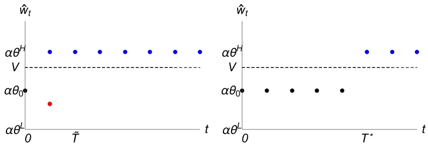
It follows that under complete evaluation the wage profile is random. Viewing the agent as a representative employee, one out of many independent draws, would result in two distinct features. First, there would be a cross-sectional variation of employees’ wage in periods before ˆT: some employees are proven to be high types and some still try to achieve a success. Second, the wage of a given employee is likely to decrease during his career in the firm. The wage profile is illustrated in Figure 1.

The players payoffs are UA_{, U}P_{≃(0.21,0.1). Note that U}A_{> V, so the agent strictly}

benefits from working at the firm as compared to his outside option.

Equilibrium evaluation Now, consider a partial evaluation policy, namely, a single revi-sion policy, mT = yT−1 and mt =∅ for t 6=T. Under this policy, the principle provides no

informative evaluations before or after the single revision date T when she conducts a full evaluation of past performance.

Under the single revision policy, the agent’s wage at the firm exhibits a single jump at the revision date. No informative evaluations are conducted before the revision time. During this period, the agent’s wage stands still at the prior level, w0 = 1/8. At the revision time,

is proven to be of a high type, and his wage jumps up to wH

T = 1/4. If no successes are

found, then the productivity expectation drops, as does the wage, towL

T = 2(1+21 T₎. After the

revision time, no informative evaluations are conducted, so the wage stays at the revision level forever.

Given the career prospects, the agent’s optimal quitting time depends on the revision date and can take only values 0 or T. Indeed, in periods after the revision, t ≥ T, the agent is essentially facing a no-evaluation policy; his wage is fixed. Consequently, because

wH

T > V > wTL, the agent immediately quits at timeT if no success is revealed; otherwise, he

stays at the firm forever. Before the revision, t < T, the agent’s continuation payoff weakly increases in t as the revision time gets closer. Hence, the agent’s quitting problem reduces to a binary choice: to either quit at time 0 or stay until the revision time and quit only if no successes are revealed.

If the revision date equals the complete evaluation time T = ˆT, then the agent prefers to stay towards the revision because this strategy delivers him payoff greater than V. In fact, this strategy delivers the same payoff as the best response to a complete evaluation policy. This is not a coincidence. Both strategies induce the same joint distribution of productivity and quitting time. They differ only in their wage profiles: before T, the wage is fixed under a revision policy and is random under a complete evaluation policy. However, because wage is a martingale, the agent receives, on average, the same wage, and, hence, the same payoff. Similarly, these strategies deliver the same payoff to the principal.

The principal can induce the agent to generate more surplus by postponing the revision until time T > Tˆ. However, there is a limit on how late the revision can be performed because the agent may prefer to quit at time 0. A maximal incentive compatible revision time can be calculated to beT∗ _{= 10.}

In fact, the revision policy with the revision time T∗ _{is optimal for the principal and,} hence, is an equilibrium evaluation policy. Indeed, it delivers payoffs UA∗ _{= V = 0.2,}

UP∗ _{≃0.12. Moreover, these payoffs are Pareto efficient because the agent never quits when} successful.Because the agent can guarantee his safe option by quitting at time 0, the principal cannot achieve payoffs above UP∗_{, and the result follows. The equilibrium wage profile is} illustrated in Figure 1. Notably, the resulting equilibrium wage profile is deterministic and weakly increasing. Effectively, it exhibits an up-or-out pattern with downward wage rigidity.

αθ0

αθL

αθH

0 V

T˜

t w_t

αθ0

αθL

αθH

0 V

T*

t w_t

Figure 1: Wage profile under complete evaluation policy (left) and equilibrium evaluation policy (right).

there are only two states or if the technology satisfies general regularity assumptions.

4

Equilibrium Analysis

Equilibrium characterization requires finding an evaluation policy optimal for the principal which is a dynamic information disclosure problem. Such problems are known to be difficult due to their dynamic structure and multidimensionality. The characterization is further complicated because the information that can be disclosed is gradually and endogenously generated, and the agent is forward looking. Because of these features, the existing techniques of Kremer, Mansour, and Perry (2014) and Ely (2017) cannot be applied.

Instead, I develop and use an efficiency approach. First, I characterize the set of Pareto-efficient payoffs (Sections 4.1, 4.2). Second, I provide an upper bound on the principal’s equilibrium payoffs. Finally, I show the upper bound can be achieved with a particular information policy (Section 4.3).

4.1

Payoff Transformation

Before characterizing the set of feasible and Pareto-efficient payoffs, it is useful to investigate the players’ payoffs. Intuitively, because both players are risk neutral, the mean-preserving spread of a wage should not affect their payoffs in any period. Hence, receiving a fixed wage proportional to the expected performance at the beginning of a period should be payoff equivalent to receiving a bonus proportional to performance at the end of a period .

Lemma 1. (Payoff Transformation) The players’ payoffs can be written as

UP _{(m, τ) =}

Em,τ

"

(1−δ)

τ−1

X

t=0

δt_(1−α)y t

#

, (10)

UA_{(m, τ) =}

Em,τ

"

(1−δ)

τ−1

X

t=0

δt_αy

t+δτV

#

. (11)

Lemma 1 implies the current setting is strategically equivalent in a sense of Thompson

(1952) to the setting of persuasion of bandit experimentation.6 _{They have the same set of} strategies and each strategy pair delivers the same payoffs to both players. Consequently, the two settings have the same feasible payoffs and equilibria. In this alternative setting, the agent sequentially pulls the arm of a slot machine and decides when to stop. Pulling the arm generates a stochastic reward, which is proportionally split between the agent and the principal. The reward depends on the machine’s type and is not observed by the agent. The principal designs what reward information the agent observes to maximize her own payoffs. Further, the payoff representation (10) and (11) highlights the nature of the conflict between the players. The principal does not have a safe option. She achieves maximal payoffs when the agent generates maximal expected surplus in the relationship. Because all types are positive, Θ ⊆ R+, it happens when the agent never quits. In contrast, the agent has a safe option. He would like to quit when his continuation payoff falls below it. Clearly, then, his payoffs are maximized when the principal provides complete evaluation because it allows him to make the most informed quitting decision.

Proposition 1. (Preferred Strategies)The principal’s payoff is maximized if the agent never quits, τ ≡ ∞, irrespective of the evaluation policy. The agent’s payoff is maximized if the principal provides complete evaluation mt≡yt−1 and the agent quits optimally.

4.2

Feasible Payoffs

I proceed with characterizing the set of feasible payoffs. Recall from standard game-theoretic terminology that a pair of strategies m ∈ M, τ ∈ T delivers payoffs uA_{, u}P _{if given the}

strategies the payoff of the agent equals touA _{and a payoff of the principal equals to u}P_{. In}

turn, payoffs uA_{, u}P

are feasible if they can be delivered by some players’ strategies. The payoffs are (weakly Pareto) efficient if there are no strategies that deliver strictly greater payoffs to both players. Denote the set of all feasible payoffs by W.

By standard arguments, the set of feasible payoffs is compact and convex. Its boundary

∂W can be characterized by the supporting hyperplane theorem. In particular, for any

payoffs uA_{, u}P_{∈∂W, there are payoff coefficients λ}A_{, λ}P _∈

Rwith at least one coefficient different from 0, such that:

uA, uP∈arg max

(uA_′,uP_′)∈Wλ

A

uA′+λPuP′. (12)

Conversely, for any payoff coefficients λA_{, λ}P _∈

R, a solution to the problem (12) belongs to the boundary ∂W. Positive agent’s payoff coefficients, λA _{> 0, correspond to the east}

boundary of W. Positive principal’s coefficients λP _{>0 correspond to the north boundary}

of W. Positive coefficients of both players λA_{, λ}P _{≥0 span all efficient payoffs.}

In other words, boundary payoffs can be delivered by some strategies that maximize dif-ferent linear combination of players’ payoffs. This maximization is equivalent to an optimal stopping problem with a modified safe option and performance value. In fact, a straight-forward application of Lemma 1 shows the problem (12) is equivalent to maximizing or minimizing payoffs of a fictitious agent with a virtual safe option V′_:

UF _{(m, τ, V}′_{) =} Em,τ

"

(1−δ)

τ−1

X

t=0

δt_αy

t+δτV′

#

. (13)

Lemma 2. (Feasible Payoffs)The set of feasible payoffsW is compact and convex. Moreover:

1. Its west boundary is delivered by (m′_{, τ}′_{)∈arg min}

m,τ UF(m, τ, V′) for V′ ≥0,

2. Its east boundary is delivered by (m′_{, τ}′_{)∈arg max}

m,τUF(m, τ, V′) for V′ ≥0, and

3. Its efficient payoffs are delivered by (m′_{, τ}′_{)∈arg max}

m,τUF(m, τ, V′) for V′ ∈[0, V].

Figure2depicts a set of feasible payoffs of the binary example in Section3.7 _PointsAandD, as well as any payoffs on the segmentAD, can be delivered by a quitting time that does not depend on evaluations. PointAcorresponds to payoffs (αθ0,(1−α)θ0) and can be delivered

by the agent never quitting, τ ≡ ∞. This is the best outcome for the principal. Point D

corresponds to payoffs (V,0) and is delivered by agent quitting at time zero, τ ≡0. This is the worst outcome for the principal. The payoffs on the segment AD can be delivered by a randomization between these two quitting times.

To obtain payoffs outside the segmentAD, the quitting time must depend on productivity through an informative evaluation policy. Roughly, to deliver payoffs to the west off AD, the strategies should use performance information in a Pareto-destructive way. In particular, the west boundary is delivered by strategies that minimize the payoff of an agent with a

7_{The shape of the feasible payoff set depends on performance technology. In general, its boundary does}

A

B

C

D

αθ0 V

(1_-α₎θ₀

0

UA UP

Figure 2: A set of feasible payoffs W. Drawn for the binary example of Section 3.

virtual safe option. In contrast, to deliver payoffs to the east off AD, the strategies should use the information in a Pareto-improving way. In particular, the west boundary can be delivered by strategies that maximize the payoff of an agent with a virtual safe option. An arc CD corresponds to virtual options V′ _{≥ V. An arc AC corresponds to virtual options} 0≤V′ _{≤V. PointC corresponds to a virtual safe option V}′ _{=V. This is the best outcome} for the agent. Point B maximizes the principal’s payoff among all payoffs that deliver at least a safe option payoff to the agent.

4.3

Equilibrium Payoffs

The notion of feasibility ignores players’ incentives. In particular, all feasible payoffs can be delivered by a complete evaluation policy because the quitting time can ignore any additional information. However, under complete evaluation, the agent would act in his own interests. He would choose a quitting time to maximize his payoff, which would correspond to point

C in Figure 2.

To incorporate the players’ incentives I refer to mechanism-design terminology and say an evaluation policym ∈ M implements payoffsuA_{, u}P _{if the payoffs are delivered by the}

policy and some agent’s best response to it. In turn, payoffs uA_{, u}P _{are implementable if}

they can be implemented by some evaluation policy.

complete-evaluation policy; that is, to send a “quit” message only after those performance histories at which the agent himself would quit. If the agent follows the recommendations, then the joint distribution of quitting time and performance will be the same. By Lemma

1, his payoff then equals the payoffs of point C. Because it is his maximal feasible payoff, he cannot do better than follow the recommendations, and so this recommendation policy would implement payoffs C.

Definition 2. An evaluation policy is a recommendation policy if it places a positive prob-ability on at most two messages: “stay” and “quit.” A recommendation policy is incentive compatible if following the recommendations is an agent’s best response.

In fact, the agent cannot do better than follow the recommendations of an arbitrary rec-ommendation policy that mimics his best response. This follows from the standard argument ofMyerson (1986). Consider an arbitrary evaluation policy m and a recommendation policy

m′ _{that mimics an agent’s best response to m. Because the agent always knows his actions,} the policy m′ _{provides weakly less information than m. Hence, his payoff cannot be higher} than that under m. Following the recommendations delivers the agent the same payoff as under m and hence is a best response to m′_.

In other words, the recommendation policies provide minimal information for the agent to make his quitting decision. The principal does not need to provide any information besides that. Note that Lemma 1 is crucial for this observation because it establishes that the net payoff effect on evaluation policy comes only through its effect on a quitting time and not on a wage.

Lemma 3. (Recommendation principle) All implementable payoffs can be implemented by incentive compatible recommendation policies.

It is instructive to compare the recommendation principle with the informativeness prin-ciple of ?. The recommendation principle states that the principal may provide minimal information to the agent. Under a recommendation policy, the agent observes only “stay” or “quit” messages without any additional performance details. In contrast, the informa-tiveness principle states that the agent’s wage should depend on the finest details of agent’s performance even when he is risk averse. This highlights the difference in focuses of the two papers. Specifically, I study a design of information for a fixed payoff structure (4), and ?

studies a design of a reward contract for a fixed information structure.

I proceed with a characterization of implementable efficient payoffs. The agent can secure the payoffV by quitting at time 0. Hence, payoffs that deliver to the agent payoffs less than

can be implemented. At the same time, point C is implementable by a complete-evaluation policy. It turns out that all efficient payoffs on the segment BC are implementable as well.

Lemma 4. (Implementable Payoffs)No payoffs withuA _{< V are implementable. All efficient}

payoffs with uA_{≥V are implementable.}

This lemma builds on the efficient payoff characterization of Lemma 2 and the recom-mendation principle of Lemma3. By the payoff characterization, the efficient payoffs can be delivered by strategies (m, τ) that maximize a payoff of an agent with a virtual safe option

V′ _{∈[0, V]. It turns out that the agent, if faced with a recommendation policy that mimics}

τ, is willing to follow recommendations. Recommendations to quit are incentive compatible because even the agent with a lower safe option is willing to follow them. Recommendations to stay are incentive compatible because the agent’s continuation payoff weakly increases with tenure.

In equilibrium, the principal chooses an evaluation policy to maximize her payoffs. Equiv-alently, the principal maximizes her payoff among all implementable payoffs. It is clear from Lemma 4 that she optimally chooses an efficient payoff that delivers V to the agent (point

B in Figure 2). The following theorem states the result formally.

Theorem 1. (Equilibrium Payoffs) Equilibrium payoffs exist and are unique and strictly efficient:

uA∗ =V, uP∗ = max

(uP_,V)∈Wu

P

.

Proof. Because the set of feasible payoffs W is compact, such payoffs uA∗_{, u}P∗

exist. By Lemma 4, uP∗ _{is an upper bound on the principal’s payoffs and can be implemented, hence}

uA∗_{, u}P∗ _{are equilibrium payoffs. Because the efficient frontier is strictly decreasing inu}A_,

there are no other equilibrium payoffs and uA∗_{, u}P∗

are strictly efficient.

5

Wage Profile

Theorem1establishes uniqueness of equilibrium payoffs. However, several equilibrium evalu-ation policies could possibly deliver these payoffs but result in different wage profiles. In what follows, I concentrate on a particular equilibrium in which the principal uses an incentive-compatible recommendation policy. By Lemma 3, this equilibrium always exists and there are at least two reasons to concentrate on it. First, the recommendation policies are mini-mally informative; any other policy can be Blackwell garbled into a recommendation policy without affecting the players’ payoffs. Providing minimal information may be desirable to avoid its misuse by the agent in ways not conceivable by the principal. Second, the recom-mendation policies minimize wage volatility; any additional information results in a mean-preserving wage split. Minimizing volatility may be desirable if the agent is (marginally) risk averse.

Definition 3. An equilibrium (m∗_{, τ}∗_{) is minimally informative if m}∗ _{is a recommendation} policy and τ∗ _{follows its recommendations.}

In a minimally informative equilibrium, the wage profile is deterministic. Indeed, in any period, there is a unique history of past evaluations that results in the agent staying at the firm; namely, a sequence of recommendations to stay. Consequently, the equilibrium agent’s career takes a particularly simple form. There is a deterministic wage profileW and commonly known performance requirements to stay at the firm. If the agent’s performance satisfies these requirements, he stays at the firm; otherwise, he quits and secures a safe option.

The equilibrium wage profile depends on the equilibrium recommendation policy, which, in turn, depends on technology details. However, by Theorem 1, the equilibrium policy is efficient. It allows me to establish wage profile properties that hold for a broad class of technologies.

5.1

Downward Wage Rigidity

Definition 4. A recommendation policy is a cutoff policy (in expectations) if there exists a cutoff function qt:Yt−1 →Rsuch that

mt=

    

"stay," if E[θ |yt−1_{]> q}

t−1(yt−2),

"quit," if _E[θ |yt−1_{]< q}

t−1(yt−2).

The naive intuition overlooks the fact that, in general, efficient selection should account for the whole profile of productivity beliefs, not just productivity expectation. Roughly, a greater productivity variance increases the chances of being highly productive and, hence, increases the option value of quitting and experimentation. An agent with a lower expected productivity but higher chances of being very productive can be worth keeping, whereas an agent with higher but certain productivity can be worth terminating. As a result, an efficient policy may not be cutoff, and the resulting equilibrium wage may decrease.

Nevertheless, I show that efficient policies are cutoff in many cases. By Lemmas 2and3, any efficient policy maximizes a payoff of an agent with some virtual safe optionV′ _{∈[0, V].} Such policy is Markov in the productivity beliefs, so the space of beliefs can be split in two sets: the set at which the agent stays and the set at which the agent quits. The exact characterization depends on parameters of the problem and can be intractable. However, it can be obtained in the following cases.

If there are only two productivity types, |Θ|= 2, then there is a threshold expectationqc

so that under any efficient policy, the agent stays if the productivity expectation is above the threshold and quits otherwise.8 _{That is, an optimal policy is cutoff with the cutoff function} being constant.

If there are more than two types, |Θ| >2, then belief is a multidimensional object, and the efficient policy can be characterized only under additional assumptions.

Definition 5. A technology isregular if it admits densities and∀θ, θ′ _{∈Θ, y, y}′ _∈suppf

θ∩

suppfθ′, θ′ > θ, y′ > y

fθ′(y′)f_θ(y)≥f_θ′(y)f_θ(y′) (MLRP).

Under the regular technology, the conditional performance distributions satisfy the monotone likelihood property. Most technologies used in the literature satisfy this condition. The regularity assumption adds structure necessary to analyze the multiple-type case. Banks and Sundaram (1992) use the regularity condition to establish that an optimal strategy is cutoff.

In both cases, in a minimally informative equilibrium, the evaluation policy is cutoff and wage profile exhibits downward rigidity. The following theorem summarizes the results.

Theorem 2. (Downward Wage Rigidity)If there are only two types|Θ|= 2or the technology is regular, then in any minimally informative equilibrium:

1. An evaluation policy m is a cutoff policy, and

2. The wage profile W is deterministic and weakly increasing.

The theorem establishes sufficient conditions under which the equilibrium wage exhibits downward rigidity. The conditions are plausible in that they are satisfied in most exist-ing models of career concerns and experimentation. Interestexist-ingly, the proof shows even a stronger statement: not only the expected productivity increases, but also the whole profile of productivity beliefs shifts upwards in an MLRP sense.

5.2

Wage Profile Shape

Theorem 2establishes that under general conditions the minimally informative wage profile is deterministic and weakly increasing. Nevertheless, the exact shape of the wage profile depends on technology details. To understand the role of technology on equilibrium, it is important to be able to calculate the wage profile.

The following algorithm builds on the results of Section4and calculates wage profile for a given technology, discount factor, and safe option. In the first step, it solves the maximization problems from Lemma 2 for all virtual safe options V′ _{∈ [0, V]. These problems can be} without loss reduced to standard optimal stopping problems by setting evaluation policy to complete evaluation. Denote the corresponding optimal stopping times ˆτ(V′_{). In the} second step, the algorithm calculates the payoffs of the agent with a safe option V if he follows ˆτ(V′_{). Denote the payoffs by ˆu}A_(V′_{). In the last step, the algorithm finds V}′ _such that ˆuA_(V′_{) = V so that the agent is left with no rents. Such V}′ _{exists because ˆu}A_(V′_{) is} continuous, ˆuA_{(V) ≥ V, and ˆu}A_{(0) = w}

0 < V. Denote the corresponding safe option by

V′∗_{. The evaluation policy that recommends ˆτ(V}′∗_{), and the agent strategy that follows} the recommendations, constitute an equilibrium by Theorem1and Lemma 3. The resulting wage profile and quitting rate can then be calculated from their definitions either in closed form or by Monte Carlo simulations.

Coarse Performance In many industries, performance measures are coarse. A lawyer performance is captured by the number of successful trials, a consultant performance is measured by outcomes of his past projects, and a drug laboratory performance is captured by the number of new drugs developed. In all these cases, a performance outcome within any period is limited to few options that cannot fully reveal productivity. As a result, productivity learning is limited, and beliefs take a limited set of values. It turns out that this can translate into discontinuity of the equilibrium wage profile and a promotion-like career consisting of infrequent performance revisions followed by either quitting or staying at a higher wage.

I illustrate with the following example. The performance is binary, low or high, Y =

n

yL_{, y}Ho_{. Without loss of generality, y}L _{= 0, y}H _{= 1. There are two equally likely types,}

Θ =nθL_{, θ}Ho_{. The type corresponds to the probability of generating high performance,}

fθ(y) yL yH

θL _1−θL _θL

θH _1−θH _θH

.

with 0 < θL _{< θ}H _{< 1 so that no performance realization is conclusive. Observing high}

performanceyH _{increases productivity expectation; observing low performancey}L _decreases

it.

Because the type is binary, as discussed in Section 5.1, an equilibrium evaluation policy is cutoff with a constant cutoff q. The cutoff is chosen so that the agent obtains a payoff

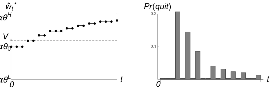
V by following the recommendations. The cutoff and the corresponding wage profile and quitting rate can be calculated by Monte Carlo simulations and presented in Figure 3.

Note how the agent’s equilibrium career can be read off these plots. The agent starts working at period 0. In the first several periods, no evaluation is conducted—performance is not sufficiently informative to bring the expectations below q. During this time, the agent’s expected productivity and, hence, the wage, stay the same. In the beginning of fourth period, the first evaluation of past performance is conducted. If the performance was sufficiently bad, in this case corresponding to few high realizations, the wage drops below q, and the agent quits. Otherwise, the wage experiences a jump, and the agent stays at the firm for at least the next few periods. Such infrequent revisions are repeated throughout the agent’s career.

em-αθ

αθ

αθ

0

V

● ● ●

● ● ● ●

● ● ● ● ● ● ● ● ●

● ● ● ●

t

w



0

t

0.1 0.2

Pr

(

quit

)

Figure 3: Wage profile (left) and quitting rate (right) in a minimally informative equilibrium. Coarse performance. Θ = nθL_{, θ}Ho_{, Y = {0,1}, Pr (y = 1|θ) = θ, α = 1/2, θ}L _{= 0.2,}

θH _{= 0.4, V = 0.6. Computed numerically by Monte Carlo simulation.}

ployees. In this case, it is possible to swing productivity expectations below the equilibrium cutoff in every period. As a result, the quitting may happen in any period, and the wage strictly increases with tenure.

I illustrate this case with the following example. Performance outcomes are rich,Y =R. There are two possible types, Θ = nθL_{, θ}Ho_{, and each type is equally likely. Performance}

is distributed according to a Gaussian distribution with fixed variance and the mean being equal to the productivity:

yt =θ+ε, ε∼N

0, σ2.

In this way, lower performance decreases expected productivity. Importantly, the perfor-mance can be very conclusive—for any prior expectation below θH_{, a probability of interim}

expectation being arbitrarily close to θL _{is positive. As a result, there is a positive selection}

in every period, and the wage is strictly increasing with tenure. The equilibrium cutoff, wage profile, and the quitting rate can be computed numerically by the algorithm and are presented in Figure4.

αθ

αθ

αθ

0

V

● ● ● ● ● ●

● ● ● ●

● ● ● ● ● ●

● ● ● ●

t

w



0

t

0.1

Pr

(

quit

)

Figure 4: Wage profile (left) and quitting rate (right) in a minimally informative equilibrium. Rich performance. Θ = nθL_{, θ}Ho_{, y}

t = θ +εt, εt ∼ N(0, σ2), σ = 0.6, α = 1/2, θL = 0,

θH _{= 1, V = 0.6. Computed numerically by Monte Carlo simulation.}

well and is likely to be a high type. Most selection happens in the middle of the career, when information sufficient to swing expectations below a cutoff has been accumulated but much productivity uncertainty remains.

6

Discussion

6.1

Wages and Career

The analysis draws attention to a role evaluations may play in explaining internal labor market dynamics. I show organizations may systematically structure their evaluations in a way that results in wage patterns observed in practice. First, in a minimally informative equilibrium, the wage is a deterministic function of tenure. That is, all workers from the same cohort receive the same salary. Second, I show the equilibrium evaluation results in downward wage rigidity. Under complete evaluation, the wage may decrease, reflecting lower expectation following bad performance. However, under equilibrium evaluation, the wage never decreases—bad evaluations are infrequent and result in immediate resignation of the employee. As bad performers quit over time, the productivity expectations and the wage of retained employees increase. Notably, the wage grows even in the absence of human capital accumulation and elaborate incentive schemes. These qualitative properties are robust in a broad class of performance technologies and not driven by specific assumptions about the production process.

Charac-terizing features of a career ladder are infrequent evaluations that result in an employee quitting the job or getting a promotion associated with a permanent wage increase. I show in Section 5.2 that this up-or-out structure can be driven by equilibrium evaluation when performance technology is coarse. The evaluation explanation is based solely on positive employee selection and does not require any increase of responsibilities or authority to come with promotion. This explanation may be particularly relevant for professional firms in which employee talents have high impact on performance and are learned gradually over time.

6.2

Evaluation Practices

My analysis provides a novel perspective on evaluation practices in organizations. First, it is commonly observed that evaluations feature rating compression and lenience bias—most employees are bunched at the highest grades with lower grades reserved for exceptionally bad performance. This feature is often attributed to behavioral biases of evaluators and criticized for lowering evaluation informativeness. However, my analysis shows these prac-tices can in fact benefit a firm. In a minimally informative equilibrium, while staying at the firm, all employees receive the same “good” grade. A “bad grade” is received only for exceptionally bad performance, which lowers the wage dramatically and leads to immediate resignation. Second, there is no agreement on whether evaluations should be retrospective, that is, account for past performance. My analysis suggests that such an accounting is gen-erally necessary. The equilibrium evaluation policy is Markov in belief; that is, it based on the whole performance history. In general, this policy cannot be implemented through a sequence of grades based solely on current performance.

The equilibrium evaluation policy can also have a psychological interpretation for main-taining workforce morale. The organizational literature has long recognized that optimal evaluation provision must balance between two opposing forces—the employee’s need for evaluation and the damage to his self-esteem. On one hand, evaluation is a valuable input for employees’ future decisions. On the other hand, any evaluation may turn out negative and discourage an employee. My model can be viewed as a formalization of these effects with the agent’s morale captured by his productivity belief.9 _{The equilibrium policy can} then be interpreted as a policy that optimally trades-off these two competing effects.

6.3

Commitment

My analysis relies on the ability of the firm to commit to its evaluation policy. In fact, several layers of commitment matter. First, I assume evaluations are objective, so that the information is verifiable. If the evaluation would be “cheap talk,” then the equilibrium recommendation policy would not be credible—the principal would always recommend the agent to stay. Second, I assume the principal commits to the evaluation rules at the beginning of the relationship and cannot change them down the road. This assumption matters because the equilibrium evaluation policy is not time consistent. Indeed, under the equilibrium policy, the only binding constraint is the participation constraint at time 0. As long as the agent stays at a firm, his continuation value increases, and his incentive constraints become slack. Hence, even if the players are symmetrically informed, the principal would like to change the evaluation policy after a recommendation to stay to extract more continuation surplus. The incentives to change the policy are even stronger if the principal can observe additional information besides evaluations. For these reasons, the equilibrium policy is not implementable without commitment. Because any equilibrium policy without commitment can be replicated with commitment, the commitment power is strictly valuable for the firm. One way for a firm to sustain evaluation commitment is to have an independent human resource department. The evaluation policy then corresponds to rules it uses in evaluating their employees, such as timing and criteria of conducting evaluations. As long as the rules are commonly known and the department is independent, the department has no incentives to not follow them. This would make the evaluations credible and allow the firm to implement the equilibrium policy.

7

Conclusion

Evaluation of individual performance is an important part of organizational life. Although much evaluation is informal, most firms have formal evaluation policies designed to collect and distribute performance information to employees. In this work, I showed an equilibrium design of these policies can explain many features of internal labor market observed in practice, including downward wage rigidity. Information control allows the organization to extract all rents from its employees and achieve a Pareto-efficient outcome despite conflict of interests.

information may not be under full control of the firm—some performance outcomes may be publicly observable. Richer monetary contracts may be available. Incorporating these features would make the model more applicable in practice and constitute a plausible venue for future work. The efficiency approach developed in this paper may facilitate analysis of these richer settings as well. In the meantime, the proposed evaluation theory could be viewed as complimenting existing theories of wage dynamics and internal labor markets.

References

Banks, J. S. and R. K. Sundaram (1992): “Denumerable-Armed Bandits,”

Economet-rica, 1071–1096.

Bergemann, D. and J. Välimäki (2008): “Bandit Problems,” in New Palgrave

Dictio-nary of Economics, ed. by S. N. Durlauf and L. E. Blume, Basingstoke, UK: Palgrave

Macmillan.

Ederer, F.(2010): “Feedback and Motivation in Dynamic Tournaments,”Journal of

Eco-nomics & Management Strategy, 19, 733–769.

Ely, J. C. (2017): “Beeps,” American Economic Review, 107, 31–53.

Ely, J. C. and M. Szydlowski (2017): “Moving the Goalposts,”Working paper.

Fang, H. and G. Moscarini(2005): “Morale Hazard,” Journal of Monetary Economics,

52, 749–777.

Gittins, J. C. and D. M. Jones(1974): “A Dynamic Allocation Index for the Sequential

Design of Experiments,” inProgress in Statistics, ed. by I. Vincze, J. Gani, and K. Sarkadi,

Amsterdam: North-Holland Pub. Co., 241–266.

Goltsman, M. and A. Mukherjee(2011): “Interim Performance Feedback in Multistage

Tournaments: The Optimality of Partial Disclosure,” Journal of Labor Economics, 29,

Guo, Y. (2016): “Dynamic Delegation of Experimentation,” American Economic Review,

106, 1969–2008.

Halac, M., N. Kartik, and Q. Liu (2016): “Optimal Contracts for Experimentation,”

Review of Economic Studies, 83, 1040–1091.

Hansen, S. E. (2013): “Performance Feedback with Career Concerns,” Journal of Law,

Economics, and Organization, 29, 1279–1316.

Holmström, B. (1999): “Managerial Incentive Problems: A Dynamic Perspective,” The

Review of Economic Studies, 66, 169–182.

Hörner, J. and Y. Guo(2015): “Dynamic Mechanisms without Money,”Working Paper.

Hörner, J. and N. Lambert (2016): “Motivational Ratings,” Working Paper.

Kamenica, E. and M. Gentzkow (2011): “Bayesian Persuasion,” American Economic

Review, 101, 2590–2615.

Kremer, I., Y. Mansour, and M. Perry (2014): “Implementing the ’Wisdom of the

Crowd’,” Journal of Political Economy, 122, 988–1012.

Murphy, K. R. and J. Cleveland (1995): Understanding Performance Appraisal:

So-cial, Organizational, and Goal-Based Perspectives, Sage.

Myerson, R. B. (1986): “Multistage Games with Communication,” Econometrica, 54,

323–358.

Orlov, D. (2016): “Optimal Design of Internal Disclosure,” Working Paper.

Orlov, D., A. Skrzypacz, and P. Zryumov (2017): “Persuading the Principal to

Wait,” Working Paper.

Rayo, L. and I. Segal (2010): “Optimal Information Disclosure,” Journal of Political

Renault, J., E. Solan, and N. Vieille (2017): “Optimal Dynamic Information

Provi-sion,”Games and Economic Behavior, 104, 329–349.

Rodina, D. (2016): “Information Design and Career Concerns,” Working paper.

Thompson, F. B. (1952): “Equivalence of Games in Extensive Form,” Technical report

8

Appendix

Proof of Lemma 1 Take any evaluation policy m and consider a stochastic processX =

{Xs}s≥1 with

Xs= (1−δ) s−1

X

t=0

δt yt−E

h

θ|mti .

The process X is a bounded martingale with respect to a filtration generated bym because

E[Xs+1 |ms] =Xs+ (1−δ)δtE[ys−E[θ|ms]|ms]

=Xs+ (1−δ)δt(E[ys |ms]−E[θ |ms])

=Xs+ (1−δ)δt(E[θ |ms]−E[θ|ms])

=Xs.

The second line follows from the law of iterated expectations and the third line follows from the productivity definition (1). It follows from the optional stopping theorem that for any stopping time τ measurable with respect to m:

E[Xτ] =E[X0] = 0.

Equivalently, by wage definition (4), for any evaluation policym and a stopping time τ,

(1−δ)Em,τ τ

X

t=0

δt_w

t= (1−δ) τ

X

t=0

δt_αy t.

The result follows.

Proof of Lemma 2. As shown in the main body of the paper all boundary payoffs can be obtained by strategies that maximize a linear combination of players’ payoffs. By Lemma1, this combination can be written as

λAUA(m, τ) +λPUP (m, τ) =Em,τ

"

(1−δ)

τ

X

t=0

δtλAα+λP(1−α)yt+δτλAV

# .

If λA_α+λP _{(1−α)>0, then maximizing the payoff combination is equivalent to}

max-imizing a payoff of an agent with a virtual safe option V′ ₌ λA_α

λA_α+λP_(1−α)V. If λA≤ 0, then

clearly τ ≡ ∞so all such coefficients correspond to payoffs (αθ0,(1−α)θ0). If λA>0, then

If λA_α+λP_{(1−α) < 0, then maximizing the payoff combination is equivalent to}

min-imizing a payoff of a an agent with a virtual safe option V′ ₌ λA_α

λA_α+λP_(1−α)V. If λA ≥ 0,

then the optimal quitting time is τ ≡0, corresponding to payoffs (V,0). IfλA_{<0, then the}

payoffs belong to the west boundary and V′ _{>0. The result follows.}

Proof of Lemma 4. Consider any efficient payoffs uA_{, u}P_{. If u}A_{< V, then the payoffs}

cannot be implemented because the agent can secure a payoff V by quitting at time 0. If uA _{≥ V, then by Lemma 2 the payoffs can be delivered through strategies (m, τ) that}

maximize a payoff of an agent with a safe option V′ _{∈[0, V]. Consider the recommendation} policy m′ _{that mimics τ. I show that m}′ _{is incentive compatible.}

Recommendations to quit are incentive compatible. If the agent is recommended to quit at time t, his wage at the firm stays constant at some level wtQ hereafter. Because the

strategy maximizes a virtual payoff, wQt ≤ V′ ≤V. Hence, the agent with a safe option V

agrees to quit as well.

Recommendations to stay are incentive compatible. Recommendation at time 0 is incen-tive compatible because it gives the agent a payoff of at least uA _{and u}A _{≥ V. Incentive}

compatibility at timet+ 1 follows from the incentive compatibility at timet. Indeed, denote by ˆUA

t the agent’s optimal continuation payoff conditional on being recommended to stay

at time t. Because the recommendation to stay is incentive compatible at time t and the recommendations to quit are incentive compatible everywhere, ˆUA

t is a convex combination

of wt, ˆUt+1A , and V,

ˆ

UtA= (1−δ)wt+δPr

mt+1 = "stay"|mt≡"stay"

ˆ

U_t+1A +δPrmt+1 = "quit"|mt ≡"stay"

V.

The agent obtains a continuation payoff V if he quits immediately so ˆUA

t ≥ V. The agent

obtains a continuation payoff wt if he never quits so ˆUtA ≥ wt. Thus, for the equality to

hold, it must be that ˆUA

t+1 ≥ UˆtA ≥ V. By forward induction, all recommendations to stay

are incentive compatible. This completes the proof.

Lemma 5. Fix V′ _{≥0, Θ =} n

θL_{, θ}Ho_{, and an arbitrary technology. Consider the following}

maximization problem:

max

m∈M,τ∈T Em,τ

"

(1−δ)

τ−1

X

t=0

δt

Ehθ |mti

+δτ_V′

# .

Then without loss of generality m≡y and the following statements are true.

2. If V′ _{< θ}L_{, then τ ≡ ∞ is uniquely optimal.}

3. If V′ _∈ h

θL_{, θ}Hi_{, then any optimal strategy τis equivalent (in terms of quitting}

distri-butions) to a cutoff quitting strategy with some fixed cutoff q∈hθL_{, θ}Hi_.

Proof. The problem is a standard bandit problem of an agent choosing between a risky arm with payoffs E[θ |mt_{] and a safe arm with a payoff V}′_{. This is a Markov decision problem} with an expected productivity ˆθt ,E[θ|yt] being a sufficient statistic for beliefs. An optimal

quitting strategy is characterized by Gittins and Jones (1974) to be an index policy. The risky arm is assigned an index ξθˆt

. The agent quits the arm as soon as the index drops below V′_{. The decision maker can arbitrarily randomize at ξ}

ˆ

θt

=V′_{. The index is}

ξθˆt

,_sup

τ

EhPτ

t=0δtE[θ|mt]|θˆt

i

EhPτ

t=0δt|θˆt

i

= sup

τ ˆ θt−θL

θH_−θLE

h Pτ