Munich Personal RePEc Archive
New Hampshire Effect: Behavior in
Sequential and Simultaneous Election
Contests
Irfanoglu, Zeynep and Mago, Shakun and Sheremeta, Roman
13 August 2015
Online at
https://mpra.ub.uni-muenchen.de/67520/
1
New Hampshire Effect:
Behavior in Sequential and Simultaneous Election Contests
Zeynep B. Irfanoglu a Shakun D. Mago b Roman M. Sheremeta c,*
a Department of Agricultural Economics, Purdue University, 403 W. State St., West Lafayette, IN 47906-2056, USA
b Department of Economics, Robins School of Business, University of Richmond, 1 Gateway Road, Richmond, VA 23173, USA
c Weatherhead School of Management, Case Western Reserve University and the Economic Science Institute, Chapman University
11119 Bellflower Road, Cleveland, OH 44106, USA
August 13, 2015
Abstract
Sequential contests are predicted to induce lower expenditure than simultaneous contests. This prediction is a result of a “New Hampshire Effect”– a strategic advantage created by the winner of the first battle. Contrary to this prediction, however, our laboratory study of the three-battle contests shows that sequential contests generate significantly higher expenditure than simultaneous contests. In case of sequential contests, we observe significant over-expenditure in
all three battles and find no evidence of the “New Hampshire Effect.” Despite the strategic
advantage, winners of the first battle make similar expenditures in the second battle as losers of the first battle. Moreover, instead of decreasing, subjects increase their expenditure in the second battle relative to the first battle. In case of simultaneous contests, subjects do not employ a uniform expenditure strategy and instead use a “guerilla warfare” strategy by focusing on only two of the three battles. We propose several explanations for these findings and discuss some implications.
JEL Classifications: C72, C73, C91, D72
Keywords: election, sequential contests, simultaneous contests, experiments
* Corresponding author: Roman Sheremeta, [email protected]
2
1. Introduction
The nomination process for the U.S. presidential election consists of a series of nationwide primary elections, beginning with the New Hampshire primary. The significance of this small New England state became entrenched in the quadrennial election politics in 1952, when Estes Kefauver defeated the incumbent President Harry Truman in the primary, leading
Truman to abandon his campaign. In 1988, all but one of George Bush’s Republican opponents
withdrew soon after the primary, and in 1992, number of Democratic Party candidates dwindled from five to two after the primary (Busch and Mayer, 2004). But just as candidates who do poorly in the New Hampshire primary frequently drop out, the lesser-known, underfunded candidates who do well in the primary suddenly become serious contenders to win the party nomination, garnering tremendous momentum both in terms of media coverage and campaign funding. In 1992, Bill Clinton, a little known governor of Arkansas did surprising well, and was labeled the “Comeback Kid” by the national media. In 2000, John McCain emerged as George
Bush’s principal challenger only after an upset victory in New Hampshire, and a similar
comeback was made by John Kerry in the 2004 primary. Controlling for other factors, Mayer (2004) finds that a win in the New Hampshire primary increases a candidate’s expected share of total primary votes by a remarkable 26.6 percent.1
The perception that New Hampshire plays a pivotal and perhaps a disproportionately large role in the presidential election (and thereby derives a wide array of political and economic benefits from that position) led many states to move up the date of their primaries.2
1 In a multi-candidate race, even a second-place finish in New Hampshire primary increases a candidate’s final vote
by 17.2 percent (Mayer, 2004). However, be noted that the winner of New Hampshire primary has not always won the party's nomination, as demonstrated by Republicans Harold Stassen in 1948, Henry Lodge in 1964, Pat Buchanan in 1996, and John McCain in 2000 and Democrats Estes Kefauver in 1952 and 1956, Paul Tsongas in 1992, and Hillary Clinton in 2008.
2 The total economic impact of 2000 primary on New Hampshire’s economy was estimated to be $264 million. The
3
‘Frontloading’ is the name given to a recent trend in the presidential nomination process in
which more and more states schedule their primaries near the beginning of the delegate selection process. Clustering of primaries took a huge leap forward in 1988 with the formation of ‘Super Tuesday’ when 16 states held their primaries on a single day in March. By 2008, 24 states held their primary on Super Tuesday held in the first week of February. In 2004, James Roosevelt, co-chair of the Democratic Party Rules Committee proclaimed, “We are moving towards a de facto
national primary.”
For obvious reasons, with naturally-occurring data, it is difficult to examine the exact impact of the two alternative electoral structures on both election outcomes and their economic efficiency. For this reason, we use a controlled laboratory experiment to compare a sequential
contest, such as the current presidential primaries, to a simultaneous contest, as reflected in a counterfactual national primary.3 Our theoretical framework is based on Klumpp and Polborn (2006). In this political contest model, candidates have to win the majority of electoral districts in order to obtain a prize – the party nomination. As in Tullock (1980) and Snyder (1989), we assume that candidates can influence the probability of winning an electoral district by their choice of campaign expenditure in that district. In case of a sequential contest, theory predicts that candidates should spend disproportionately larger amounts in the earlier districts than in the later districts. This difference in expenditure is attributed to the “New Hampshire Effect.” That is, the outcome of the first election creates asymmetry between ex-ante symmetric candidates in terms of their incentive to spend resources in the next district, which in turn, endogenously
presidential nomination process (Busch and Mayer, 2004). Originally held in March, the date of the New Hampshire primary has been moved up repeatedly to maintain its status as first (a tradition since 1920). In fact, the state law requires that its primary must be the first in the nation.
3 Our experiment compares two extreme benchmarks: a completely sequential contest to a completely simultaneous
contest. Present day primary system, however, has a mixed temporal structure. The nomination process starts with a series of sequential elections held in various states (Iowa caucus, New Hampshire primary, etc.) followed by days
4
increases the probability that the winner of the first district will win in subsequent districts and attain the final prize. For example, in a sequential contest with three districts (battles), the winner of the first battle wins the overall contest with probability of 0.875.4 Furthermore, the intense concentration of expenditure in the initial battles entails that there is a 0.75 probability that the contest will end in only two battles. In contrast, in case of a simultaneous contest, candidates are predicted to spend equal amounts of resources in all three battles, and this leads to complete rent dissipation if the number of battles is sufficiently large. Thus, an important consequence of this temporal difference in contest design is that the sequential contest is predicted to induce lower expenditure than the simultaneous contest, which potentially could explain why political parties may choose the sequential electoral structure of the primaries in order to minimize wasteful campaign expenditure.5
These predictions, however, are not supported in our laboratory study of the three-battle contests. In the laboratory, we find that sequential contests generate significantly higher expenditure than simultaneous contests. In case of sequential contests, we observe significant over-expenditure in all three battles and find no evidence of the “New Hampshire Effect.” Despite the strategic advantage, winners of the first battle make similar expenditures in the
4 This probability increases as the total number of battles in the contest increases.
5 The contest model is complementary to the voters’ participation model (Morton and Williams, 1999; Battaglini et
al., 2007). In the voters’ participation model the probability of winning an electoral district by a candidate depends on the number of votes received, while in the contest model such a probability depends on the relative campaign expenditure by each candidate in that district. The complementarity between the two models arises because one of the reasons for the “New Hampshire Effect” that is commonly discussed in political science is information aggregation, which is implicit in voting models. For instance, Morton and Williams (1999) compare sequential and simultaneous voting and find that in sequential voting later voters use early outcomes to infer information about asymmetric candidates, and thus make better informed choices that reflect their true preferences. Battaglini et al. (2007) find that sequential voting aggregates information better than simultaneous voting and is more efficient in some information environments, but sequential voting is inequitable because early voters bear more participation costs. By assuming that both candidates are symmetric and by abstracting from costly voter participation decision,
we are able to isolate on how candidates’ relative expenditure alone determines the likelihood of winning current and future electoral districts. That is, we examine the “New Hampshire Effect” resulting solely from candidates’
5
second battle as losers of the first battle. Moreover, instead of decreasing, subjects increase their expenditure in the second battle relative to the first battle. In case of simultaneous contests, subjects do not employ a uniform expenditure strategy and instead use a “guerilla warfare” strategy by focusing on only two of the three battles. Finally, we find that although subjects learn to behave more in line with equilibrium predictions in both types of contests, their behavior differs substantially from predictions even in the last periods of the experiment.
6
multi-battle contests in the simplest possible framework using laboratory data, which is untainted from the various complicating factors that plague naturally-occurring data, we provide a direct empirical test of the theoretical model of primary elections by Klumpp and Polborn (2006). A theory that performs well in the laboratory may not have complete external validity, but it does pass what Smith (1982) refers to as a “nontrivial test.”
The rest of the paper is organized as follows. In Section 2, we provide a brief review of the multi-battle contest literature, both theoretical and experimental. Section 3 presents our theoretical framework and Section 4 describes the experimental design, procedures and hypotheses. Section 5 reports the results of our experiment and Section 6 concludes.
2. Literature Review
The theoretical literature on multi-battle contests originated with seminal work by Fudenberg et al. (1983) and Snyder (1989).6 Fudenberg et al. (1983) model R&D competition as a sequential multi-battle contest, while Snyder (1989) models political campaigning as a
simultaneous multi-battle contest.7 For a comprehensive review of the theoretical literature on multi-battle contests see Kovenock and Roberson (2012). Klumpp and Polborn (2006) directly compare sequential and simultaneous multi-battle contests in a context of primary elections. They show that sequential contest creates a strategic advantage for the winner of the first battle, the result they call a “New Hampshire Effect,” thus minimizing potentially wasteful expenditures
in future battles.
6 One could also argue that the original formulation of a Colonel Blotto game by Borel (1921) is a starting point of
the multi-battle contest literature.
7 Building on these models, subsequent papers investigated the ramification of various factors such as the sequence
7
We conduct an experiment to test the predictions of the theoretical model by Klumpp and Polborn (2006). While most of the existing experimental studies focus on single-battle contests, recently there has been an increased interest in examining multi-battle contests. For a comprehensive review of the experimental literature on contests see Dechenaux et al. (2015). Experimental studies on simultaneous multi-battle contests have examined how different factors such as budget constraint (Avrahami and Kareev, 2009; Arad and Rubinstein, 2012; Mago and Sheremeta, 2014), information (Horta-Vallve and Llorente-Saguer, 2010), contest success function (Chowdhury et al., 2013), asymmetry in resources and battles (Kovenock et al., 2010; Arad, 2012; Holt et al., 2015) impact individual behavior in contests.
Experimental studies on sequential multi-battle contests have examined the impact of contest structure (Deck and Sheremeta, 2012), carryover (Schmitt et al., 2004), fatigue (Ryvkin, 2011), the length of the contest (Zizzo, 2002; Deck and Sheremeta, 2015), intermediate prizes and luck (Mago et al., 2013) on behavior in dynamic contests.8 Most of these studies find support for the comparative statics predictions (see the review by Dechenaux et al., 2015), but often report significant over-expenditure of resources (also known as overbidding or over-dissipation) relative to the Nash equilibrium prediction (see the review by Sheremeta, 2013).
Our study is the first to compare sequential and simultaneous multi-battle contests. Consistent with the previous studies, we find significant over-expenditure relatively to Nash equilibrium in both contests. However, our most surprising result is the reversal of the comparative statics prediction of Klumpp and Polborn (2006) – we find that contrary to prediction, the sequential contest generates higher expenditure than the simultaneous contest. This is surprising because, as mentioned above, almost all contest experiments in the literature
8 Related to the studies on sequential multi-battle contests are the studies examining multi-battle elimination contests
8
find strong support for the comparative statics predictions even if the precise quantitative predictions are refuted. We discuss several explanations for this finding in Section 5, including the sunk cost fallacy and the non-monetary utility of winning.
3. Theoretical Model
Consider a game in which two risk-neutral and equally-skilled players, 𝑋 and 𝑌, compete in a multi-battle contest for an exogenously determined and commonly known prize v. There are
𝑛 battles in the contest. Let 𝑥𝑖 and 𝑦𝑖 denote the amount of resource expenditures by players 𝑋
and 𝑌 in battle 𝑖. Following Tullock (1980), the probabilities of winning battle 𝑖 by players 𝑋 and
𝑌 are defined by contest success functions:
𝑝𝑋𝑖(𝑥𝑖, 𝑦𝑖) = 𝑥𝑖 𝑟 𝑥𝑖𝑟+𝑦
𝑖𝑟 and 𝑝𝑌𝑖(𝑥𝑖, 𝑦𝑖) = 𝑦𝑖𝑟 𝑥𝑖𝑟+𝑦
𝑖𝑟 (1)
The parameter 𝑟 in these contest success functions can be interpreted as the ‘marginal return to
lobbying outlays’ (Nitzan, 1994). When 𝑟 = 1, as assumed in this study, we have a ‘lottery’
contest wherein a player’s probability of winning the battle depends on his expenditure relative to the total expenditure.
The player who wins a majority of the battles, i.e., at least (𝑛 +1)/2 battles wins the overall contest and receives the prize 𝑣. Therefore, the net payoff of player 𝑋 (similarly for player 𝑌) is equal to the value of the prize (if he wins) minus the total expenditure he has spent during the contest:
𝜋𝑋 = {𝑣 − ∑ 𝑥𝑖 𝑛
𝑖=1 if 𝑋 wins the contest
− ∑𝑛𝑖=1𝑥𝑖 otherwise (2)
9
𝑛 =3. It is important to emphasize that all the comparative statics predictions derived in this
simplified version of the model hold for any 𝑟 ∈ (0,1] and 𝑛 ≥3 (Klumpp and Polborn, 2006). However, for our experiment we chose specific parameters of 𝑟 =1 and 𝑛 =3 to simplify the experimental environment and to facilitate greater subject comprehension.
3.1. Sequential Multi-Battle Contest
In the sequential multi-battle contest, players simultaneously choose expenditure levels
𝑥1 and 𝑦1 in battle 1. After determining the winner of battle 1, they move on to battle 2 where
they choose expenditures 𝑥2 and 𝑦2. Players continue to compete until one player accumulates the requisite two victories. The solution concept we consider is the subgame perfect Nash equilibrium. Using backward induction, we begin our examination with the final and decisive battle 3. Note that if one of the players has already won the previous two battles there is no need to compete in battle 3 and thus expenditures are 𝑥3∗ = 𝑦3∗ = 0. However, if each player has won one of previous two battles then the winner of the contest is determined by the result of battle 3. In such a case, player 𝑋’s expected payoff (similarly for player 𝑌) is equal to the probability of player 𝑋winning battle 3 𝑝𝑋3(𝑥3, 𝑦3) times the prize valuation 𝑣 minus cost of expenditure 𝑥3:
𝐸(𝜋𝑋3) = 𝑝𝑋3(𝑥3, 𝑦3)𝑣 − 𝑥3 = 𝑥3𝑥+𝑦3 3𝑣 − 𝑥3 (3)
In the unique, symmetric subgame perfect Nash equilibrium, the expenditures are 𝑥3∗ =
𝑦3∗ = 𝑣/4 and the expected payoffs are 𝐸∗(𝜋𝑋3) = 𝐸∗(𝜋𝑌3) = 𝐸∗(𝜋3) = 𝑣/4. Both players have
10
Going backwards to battle 2, suppose player 𝑋 won battle 1 and is leading the contest. Therefore, players are necessarily asymmetric, wherein player 𝑋 needs to win only one more battle to win the contest, while player 𝑌 needs to win two battles. In this case, players 𝑋 and 𝑌 have the following expected payoffs:
𝐸(𝜋𝑋2) =𝑥2𝑥+𝑦2 2𝑣 +𝑥2𝑦+𝑦2 2𝐸∗(𝜋3) − 𝑥2 and 𝐸(𝜋𝑌2) =𝑥2𝑦+𝑦2 2𝐸∗(𝜋3) − 𝑦2 (4)
These payoff profiles reflect the fact that although winning the overall contest has the same value to both players, player X’s value of winning battle 2 is higher than that of player Y. The outcome of battle 1 has an asymmetric effect on the effort choices of ex-ante symmetric players. Consequently, in battle 2 player X chooses higher expenditure than player Y, and is more likely to win the overall contest. Klumpp and Polborn (2006) call this outcome the “New
Hampshire Effect.” In the Nash equilibrium of this subgame, players choose expenditures 𝑥2∗ =
9𝑣/64 and 𝑦2∗ =3𝑣/64 which yield them expected payoffs 𝐸∗(𝜋𝑋2) =43𝑣/64 and 𝐸∗(𝜋𝑌2) =
𝑣/64.
Finally, going back to battle 1, the players are symmetric again. Both players need to accumulate two battle victories to win the contest. In this case, player 𝑋 (similarly, player 𝑌) maximizes the following expected payoff:
𝐸(𝜋𝑋1) =𝑥1𝑥+𝑦1 1𝐸∗(𝜋𝑋2) +𝑥1𝑦+𝑦1 1𝐸∗(𝜋𝑌2) − 𝑥1 (5)
In the Nash equilibrium of this subgame, players choose expenditures 𝑥1∗= 𝑦1∗ = 21𝑣/128 and earn the expected payoffs 𝐸∗(𝜋𝑋1) = 𝐸∗(𝜋𝑌1) = 𝐸∗(𝜋1) =23𝑣/128. Both players
11
players exert greater effort in that decisive battle compared to the earlier battles. Aggregating across all three battles, the expected equilibrium expenditure by each player is 41𝑣/128.
3.2. Simultaneous Multi-Battle Contest
In the simultaneous multi-battle contest, players simultaneously choose expenditure levels 𝑥𝑖 and 𝑦𝑖 for all three battles 𝑖 =1, 2, 3. Then, the winner of each individual battle is determined and the player who wins at least two battles wins the overall contest and obtains the prize. Note that each battle of the multi-battle contest is an ‘independent’ lottery contest. Therefore, player 𝑋 (similarly, player 𝑌) maximizes the following expected payoff:
𝐸(𝜋𝑋) = [(33)(𝑥+𝑦𝑥 ) 3
+ (32)(𝑥+𝑦𝑥 ) 2
(𝑥+𝑦𝑦 )] 𝑣 − 3𝑥 = [(𝑥+𝑦𝑥 )3+ (𝑥+𝑦)3𝑥2𝑦3] 𝑣 − 3𝑥 (6)
In the unique Nash equilibrium, both players make the same expenditure in all battles, i.e., 𝑥𝑖∗ = 𝑦𝑖∗= 𝑣/8 for all 𝑖.9 Aggregating across all three battles, the expected equilibrium expenditure by each player is 48𝑣/128.
4. Experimental Environment
4.1. Experimental Design and Hypotheses
We employ two treatments: sequential and simultaneous. In the sequential treatment two players compete in a sequential multi-battle contest, while in the simultaneous treatment two players compete in a simultaneous multi-battle contest. Table 1 summarizes the equilibrium predictions in both treatments for 𝑣 =100, 𝑟 = 1 and 𝑛 =3. These predictions motivate the following three hypotheses:
12
Hypothesis 1: Total expected expenditure in the sequential contest is lower compared to the simultaneous contest.
The expected total expenditure by a player in the sequential contest is 32.4, and in the simultaneous contest is 37.5.
Hypothesis 2: In the sequential contest, winner of battle 1 is more likely to win battle 2 and the overall contest.
In the sequential contest, the outcome of battle 1 creates asymmetry between ex-ante symmetric players. This asymmetry endogenously triggers differing expenditure levels in the subsequent battles and generates momentum for the winner of battle 1, also known as the “New Hampshire Effect.” Since it is less likely for the loser of battle 1 to win the contest, the absolute level of expenditures fall sharply after the outcome of battle 1 is known. In battle 2, the winner of battle 1 exerts three times more expenditure than the loser. As a result, sequential contest ends after two battles with probability 0.75, and the winner of battle 1 wins the overall contest with probability 0.875.
Hypothesis 3: In the simultaneous contest, expenditures are uniformly distributed across all three battles.
Since all three battles are identical in the simultaneous contest, both players make the same expenditure of 12.5 in each battle. This is in sharp contrast to the sequential contest where expenditures are predicted to be more intensely concentrated in the first battle.10
10 In the sequential contest, the total expected expenditure by both players in battle 1 is 32.8; in battle 2 is 18.8; and
13
4.2. Experimental Procedures
A total of seventy two subjects participated in six sessions (12 subjects per session). All subjects were undergraduate students at Chapman University and inexperienced in this decision-making environment. No one participated in more than one session. The experimental sessions were run using computer software z-Tree (Fischbacher, 2007). Throughout the session, no communication between subjects was permitted, and all choices and information were transmitted via computer terminals.11 At the beginning of each session, subjects received an initial endowment of $20 to cover any potential losses.
Each experimental session corresponded to 20 periods of play in one of the two treatments. Thus, three sessions featured the sequential treatment and three sessions featured the simultaneous treatment. Subjects were given the instructions, available in the Appendix, at the beginning of the experiment, and these were read aloud by the experimenter. Before the start of the experiment, subjects completed a computerized multiple choice quiz to verify their understanding of the instructions.12 The experiment started only after all subjects completed the quiz and explanations were provided for any incorrect answers. In every period, subjects were randomly and anonymously placed into 6 groups with 2 players in each group. To keep the terminology neutral, in the instructions we describe the task as one of making bids in boxes and the player who wins 2 boxes gets the prize of 100 experimental francs. All subjects were informed that increasing their bid would increase their chance of winning; and that regardless of who wins the prize, all subjects would have to pay their bids. In the simultaneous treatment
11 Our subject pool comprised a large number of females (67%), and the median age was 19. Although on average,
most subjects had taken two Business and Economics classes; their declared ‘major’ field of study is diverse.
12 Subjects also made 15 choices in simple lotteries, similar to Holt and Laury (2002), at the beginning of the
14
subjects were asked to make bids in three battles simultaneously. They were not allowed to bid more than 100 francs in any battle and money spent on bidding was subtracted from the initial endowment of $20.13 After subjects submitted their bids, the computer displayed own bids,
opponent’s bids, the winner of each battle, the overall winner and own final payoff. In the
sequential treatment subjects made their bidding decision sequentially, either in two or three rounds (with bids not exceeding 100 francs in any round). At the end of each round, the
computer displayed own bid, opponent’s bid, and the winner of the battle in that round. The
period ended when one of the subjects in the group won two rounds. At the end of each period, subjects were randomly re-grouped to form a new two-person group.
At the end of the experiment, 2 out of 20 periods were randomly selected for payment.14 The sum of the earnings for these 2 periods was exchanged at rate of 25 experimental francs = US$1. On average, the experimental sessions lasted for about 60 minutes, and subjects earned $21 which was paid anonymously and in cash.
5. Results
5.1. General Results
Table 2 presents the aggregate mean expenditure and payoff in both sequential and simultaneous contests. The average total expenditure is 60.8 in the sequential contest and 38.1 in the simultaneous contest. While the observed expenditure in the simultaneous contest is not significantly different from the equilibrium predictions (38.1 versus 37.5, p-value = 0.65), the observed expenditure in the sequential contest is significantly higher than predicted (60.8 versus
13 100 francs is substantially higher than the highest possible equilibrium bid, but we decided not to constrain
individual bidding to be consistent with the theoretical model which assumes no budget constraints. Additionally, we wanted to avoid potential unintended behavioral consequences since enforcing even non-binding budget constraints can unexpectedly affect subjects’ behavior (Price and Sheremeta, 2011; Sheremeta, 2011).
15
32, p-value < 0.01).15 Moreover, this over-expenditure in the sequential contest is observed in all three battles.
Finding 1: Average total expenditure in the simultaneous contest conforms to the theoretical predictions, but there is significant over-expenditure in the sequential contest.
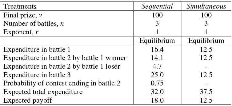
The experiment lasted for 20 periods and it is relevant to examine how expenditure evolves over the length of the experiment. Figures 1 and 2 show that in both sequential and simultaneous contests, the total expenditure decreases over time. For instance, in the sequential contest the average total expenditure in period 1 is 85.6 and it drops to 53.2 in the last period. Similarly, in the simultaneous contest the average total expenditure drops from 48.0 to 35.8. A panel regression of the total expenditure on a time trend shows that this negative relationship is significant for both contests, albeit marginally for the simultaneous contest (p-value < 0.01 in the sequential contest and p-value = 0.08 in the simultaneous contest). Our result that over-expenditure decreases with repetition in the direction of equilibrium play is consistent with previous experimental findings on single-battle contests (Davis and Reilly, 1998; Sheremeta and Zhang, 2010; Price and Sheremeta, 2011, 2015; Chowdhury et al., 2014; Mago et al., 2015).
A comparison across the two treatments informs our Hypothesis 1 that the aggregate expenditure is lower in the sequential contest relative to the simultaneous contest (32 vs 37.5). Contrary to this prediction, however, we find that the average expenditure in the sequential contest is higher than in the simultaneous contest (60.8 versus 38.1). A panel regression of total expenditure on the treatment dummy variables and a time trend indicates that this difference is
15 To support these conclusions we estimated a panel model for each treatment. We have 720 observations for each
16
significant (p-value < 0.01).16 The difference between the two contest structures remains significant even if we focus on the last 10 periods of the session (p-value = 0.03). It is important to emphasize that the magnitude of the difference between the two treatments is quite substantial in size. The sequential contest generates 60% higher expenditure than the simultaneous contest, instead of the predicted 20% lower expenditure. As a result of this over-expenditure, the observed average payoff in the sequential contest is negative and lower than prediction (-10.9 versus 18). On the other hand, the average payoff in the simultaneous contest is positive and very close to prediction (11.9 versus 12.5).
Finding 2: Average total expenditure is significantly higher in the sequential contest than in the simultaneous contest (evidence against Hypothesis 1).
Next, we take a closer look at the individual battle behavior in both sequential and simultaneous contests.
5.2. Sequential Contests
One of our central predictions is that the sequential contest generates the “New Hampshire Effect,” so that the winner of battle 1 is more likely to win battle 2 and the overall contest (Hypothesis 2). For our parameters, the winner of battle 1 is predicted to win the overall contest with probability 0.875. In the experiment, we find that the winner of battle 1 wins the overall contest with probability 0.8, and this is significantly higher than the probability of winning by the loser of battle 1 (p-value < 0.01).17 This result persist through all 20 periods of the experiment and there is no discernible time trend, as evident in Figure 3.
16 A random effects error structure accounted for the multiple decisions made by individual subjects and standard
errors were clustered at the session level to account for the session effects.
17 To support this conclusion we estimated a panel probit model for the sequential treatment, where the dependent
17
It is important to recognize, however, that our result that the winner of battle 1 is more likely to win the overall contest is not a conclusive evidence of the “New Hampshire Effect.” A best of three coin‐toss model would also generate a probability of 0.75 that the winner of battle 1 wins the overall contest. In fact, the binomial test of proportions indicates that we cannot reject the null hypothesis that the observed probability of 0.8 is significantly different from the predicted coin-toss result of 0.75 (p-value = 0.02 for probability of 0.75).18 Thus, although the winner of the battle 1 is more likely to win the overall contest, we cannot conclude with certainty that this arises due to the “New Hampshire Effect.”
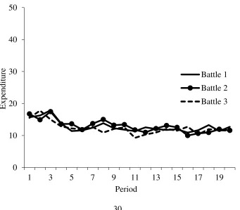
Furthermore, the individual battle behavior characterizing the effect is also not observed in the data. The theory motivating the “New Hampshire Effect” entails that winning battle 1 creates asymmetry, leading the winner of battle 1 to spend three times more in battle 2 than the loser of battle 1. More specifically, for our parameters, theory predicts that the winner of battle 1 should spend 14.1 in battle 2 and the loser of battle 1 should spend 4.7 in battle 2 (see Table 1). Contrary to these predictions, we find that the average expenditure in battle 2 by battle 1 winner is 28.5, and this is not significantly different than the average expenditure in battle 2 of 23.5 by battle 1 loser (p-value = 0.28). Moreover, instead of decreasing expenditure from 16.4 in battle 1 to 14.1 in battle 2, battle 1 winner increase expenditure from 26.7 to 28.5, with 82% of expenditures in battle 2 being higher than the equilibrium prediction of 14.1 (see Figure 4). Similarly, instead of decreasing expenditure from 16.4 in battle 1 to 4.7 in battle 2, battle 1 loser increase expenditure from 17.8 to 23.5, with 79% of expenditures in battle 2 being higher than the equilibrium prediction of 4.7. As a result, contrary to the theoretical predictions, we find that
and a dummy variable of whether the player won the first battle. The model included a random effects error structure, with the individual subject as the random effect, to account for the multiple decisions made by individual subjects. Based on estimation results, the dummy variable for win in battle 1 is significant (p-value < 0.01).
18 The null hypothesis that the observed probability is equal to 0.75 also cannot be rejected based on the
18
expenditures in battle 2 are greater than in battle 1 (value < 0.01 for battle 1 winner and p-value = 0.08 for battle 1 loser). Moreover, the aggressive over-expenditure behavior carries over to the decisive battle 3. In the final battle, average expenditure by both players is higher than the theoretical prediction of 25 (p-value < 0.01).19 Our observation of over-expenditure in all three battles is inconsistent with the theoretical predictions of the model, but it can explain why the sequential contests generate much a higher total expenditure than the simultaneous contests (Finding 2).
Aggressive play by battle 1 loser also explains why the sequential contest lasts longer than expected. Contrary to the theoretical prediction that the sequential contest should end battle 2 with probability 0.75, we find that on average the contest ends in battle 2 with probability 0.61 (see Figure 3). This difference is significant at the 1% level. However, there is some evidence of learning since the likelihood of battle 2 being the decisive one is increasing with the repetition of the experiment. For example, in the first 10 periods 56% of the contests conclude after two battles, and this proportion increased to 66% in the last 10 periods of the experiment.
Finding 3: In the sequential contest, over-expenditure is observed in all three battles. Contrary to prediction, battle 1 winner and battle 1 loser make similar expenditures in battle 2. Also, instead of decreasing their expenditure in battle 2 relative to battle 1, both battle 1 winner and battle 1 loser increase their expenditure. This results in lower probability of the contest ending in battle 2. Taken together, we do not find evidence of the “New Hampshire Effect” (evidence against Hypothesis 2).
19 The statistical tests are based on the estimation of a panel regression, similar to footnotes 15, 16 and 17. Details
19
There are several possible explanations for the significant over-expenditure observed in the sequential contest.20 One explanation is that subjects fall prey to the sunk cost fallacy (Staw, 1976). The payoff maximization problem underlying the multi-battle sequential contest equilibrium regards the expenditure in previous battles as sunk cost, and therefore ignores them. However, evidence from various behavioral studies suggests otherwise. Friedman et al. (2007) state that there are at least two distinct psychological mechanisms that might create an irrational regard for sunk cost. One mechanism is cognitive dissonance (Festinger, 1957) or self-justification (Aronson, 1968), which induces people who have sunk resources into an unprofitable activity to irrationally revise their beliefs about the profitability of an additional expenditure, in order to avoid the unpleasant acknowledgment that they made a mistake. In our experiment, subjects who get to battle 3 have already made some expenditure in the previous two battles. If the sunk cost hypothesis is true, it should entail that subjects who spend more resources in battle 1 and battle 2 are also more likely to spend more in the final decisive battle 3 – to increase their chance of winning the prize and recoup some of their expenditure. A simple
random effect regression shows a positive relationship between the expenditure in battle 3 and the total expenditure in the previous two battles (p-value = 0.06). Extending it temporally, cognitive dissonance would imply that the observed decline in expenditure in battle 1 and battle 2 over periods is associated with a similar decline in expenditure in battle 3. Data summarized in Figure 1 clearly supports this conjecture. Second mechanism underlying sunk cost relates to the prospect theory – specifically to a fixed reference point and loss-aversion (Kahneman and Tversky, 1979). This also postulates that subjects who spent more in previous battles should spend more in the current battle to avoid potential losses. We find that expenditure in battle 2 is
20 Sheremeta (2013, 2015) provides an overview of possible explanations for the over-expenditure phenomena in
20
positively related to expenditure in battle 1, both for battle 1 winner (p-value = 0.06) and battle 1 loser (p-value = 0.01). This suggests that loss-aversion can also explain why losers of battle 1 do not decrease their expenditure, but instead, increase their expenditure in battle 2 in an attempt to reduce the probability of a future loss.
over-21
expenditure (Sheremeta, 2010a, 2010b; Cason et al., 2011, 2012; Price and Sheremeta, 2011, 2015; Brookins and Ryvkin, 2014; Mago et al., 2015).21
Utility of winning may also provide insight into why expenditure is significantly higher in sequential contests compared to simultaneous contests (Finding 2). Both Parco et al. (2005) and Sheremeta (2010b) suggest that the utility of winning is increasing in the number of stages. Although the number of battles is identical in both simultaneous and sequential contest, in the sequential contest subjects can receive non-pecuniary utility of winning up to two times (when each battle winner is announced) while in the simultaneous contest such utility is received only once (when the overall winner is announced).
5.3. Simultaneous Contests
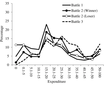
For the simultaneous contest, theory predicts that subjects allocate expenditure equally across all the three battles (Hypothesis 3). Our data reveals that although the average expenditure in all three battles is close to the predicted level of 12.5 (Table 2), none of the subjects who participated in the simultaneous contest employ a uniform expenditure strategy. Most subjects vary their expenditure between battles, with the difference from the mean expenditure across all three battles averaging at a steep 11.3. Figure 5 displays the average difference from the mean expenditure across all three battles in a given period. A lower magnitude of dispersion implies a more uniform expenditure strategy and obviously, in equilibrium, the magnitude of dispersion should be zero. We find that although there is some evidence that the dispersion of expenditure across the three battles decreases in the first five periods of the experiment; on the whole, the
21 Parco et al. (2005, pg. 328) argue that this non-pecuniary gain “may particularly apply to inexperienced subjects
for whom winning is a reward by itself.” Accordingly, in the experiment, we find that expenditure in battle 2 by
22
average difference in expenditure between battles remains positive and significant over the entire length of the experiment.
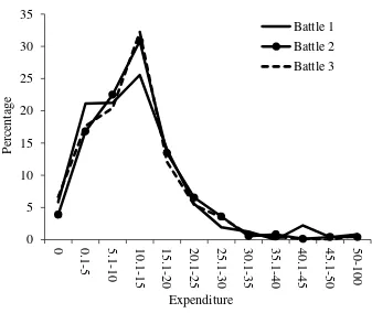
Figure 6 displays the distribution of expenditure within each battle over all 20 periods of the simultaneous contest. Two things stand out. First, despite the large variance, the overall distribution of expenditure is remarkably similar in the three battles indicating no preferential bias between battles.22 Second, more importantly, subjects’ expenditures are distributed over the entire strategy space, which is clearly inconsistent with play at a unique pure strategy Nash equilibrium. While a large majority of the expenditure is centered close to the equilibrium prediction of 12.5, there is also substantial variation in expenditure. Expenditure in an individual battle is less than 5 or more than 20, on average, 24 percent and 12 percent of the time.
Finding 4: Subjects in the simultaneous contest do not employ a uniform expenditure strategy. There is substantial dispersion in expenditure both between-battles in a given period and within-battles over time.
This dispersion in expenditure (both between and within battles) alludes to a strategy akin to “guerilla warfare.” To win the overall contest, a player needs to win a minimum of two battles. She does not derive any additional utility from winning all three battles. This suggests that players can randomly select and focus their expenditure on just two battles. We find that the average minimum expenditure in a battle is 7.5, almost half the prediction of 12.5. Indeed, 22% of time, expenditure in one of the battles is less than or equal to 1. Similarly, expenditure in the remaining two battles averages at 15.3, and exceeds the equilibrium prediction more 58% of the time. This guerilla warfare strategy (i.e., incomplete and inequitable coverage of battles) can also explain why the overall expenditure in the simultaneous contest is close to the theoretical
22 That is, there is no allocation bias such as that observed in Colonel Blotto games (Chowdhury et al., 2013), where
23
predictions (Finding 1), while it is well documented that in a single-battle contest subjects consistently overbid relative to predictions (see the review by Sheremeta, 2013).
6. Conclusion
In this study we use a laboratory experiment to compare sequential and simultaneous contests, where candidates have to win the majority of battles in order to obtain a prize. Candidates influence the probability of winning a battle by their choice of expenditure in that battle. We find that, contrary to prediction, sequential contests generate substantially higher expenditure than simultaneous contests. In sequential contests, although winners of the first battle win the overall contest more often than the losers of the first battle, we do not find conclusive evidence of the “New Hampshire Effect.” This is mainly because in sequential contests, contrary to prediction, winners and losers of the first battle make similar expenditures in the second battle. Moreover, instead of decreasing, subjects increase their expenditures in the second battle relative to the first battle. In simultaneous contests, subjects do not employ a uniform expenditure strategy and instead use a “guerilla warfare” strategy.
24
expenditure. Thus, we provide evidence that attempts such as ‘Frontloading’ and ‘Super
Tuesday’ to make presidential nomination process more like the simultaneous contest may
indeed lead to a more efficient and significantly less costly electoral process.
Our theoretical construct is a prototype model of a strategic multi-dimensional resource allocation game (Kovenock and Roberson, 2012). Although our experimental design is built around the theoretical model of Klumpp and Polborn (2006), who compare sequential and simultaneous multi-battle contests in the context of primary elections, our design can also be used to analyze problems in various fields such as military and systems defense (Hausken, 2008), advertising resource allocation (Friedman, 1958), and research and development portfolio selection (Clark and Konrad, 2008).
25
References
Altmann, S., Falk, A. & Wibral, M. (2012). Promotions and Incentives: The Case of Multistage Elimination Tournaments. Journal of Labor Economics, 30, 149-174.
Amegashie, J.A., Cadsby, C.B., & Song, Y. (2007). Competitive burnout: Theory and experimental evidence. Games and Economic Behavior, 59, 213-239.
Arad, A. & Rubinstein, A. (2012). Multi-Dimensional Iterative Reasoning in Action: The Case of the Colonel Blotto Game. Journal of Economic Behavior and Organization, 84, 571-585. Arad, A. (2012). The Tennis Coach Problem: A Game-Theoretic and Experimental study. The
B.E. Journal of Theoretical Economics, 12, 10.
Aronson, E. (1968). Dissonance Theory: Progress and Problems. In R. Abelson et al, Eds, Theories of Cognitive Consistency: A Sourcebook, Rand McNally and Co, pp. 5-27.
Avrahami, J., & Kareev, Y. (2009). Do the Weak Stand a Chance? Distribution of Resources in a Competitive Environment. Cognitive Science, 33, 940-950.
Baik, K. & Lee, S. (2000).Two-stage rent-seeking contests with carryovers. Public Choice, 103, 285-296.
Battaglini, M., Morton, R.B., & Palfrey, T.R. (2007). Efficiency, equity and timing of voting mechanisms. American Political Science Review, 101, 409-424.
Borel, E. (1921). La theorie du jeu les equations integrales a noyau symetrique. Comptes Rendus del Academie. 173, 1304-1308; English translation by Savage, L. (1953). The theory of play and integral equations with skew symmetric kernels. Econometrica, 21, 97-100.
Brookins, P., & Ryvkin, D. (2014). An experimental study of bidding in contests of incomplete information. Experimental Economics, 17, 245-261.
Busch, A., & Mayer, W. (2004). The Front-Loading Problem. In: Mayer, W. (Eds.), The making of the presidential candidate. Rowman and Littlefied Publishers, Inc, USA, 83-132.
Callander, S. (2007). Bandwagons and Momentum in Sequential Voting. Review of Economic Studies, 74, 653-684
Cason, T.N., Masters, W.A. & Sheremeta, R.M. (2011). Winner-Take-All and Proportional-Prize Contests: Theory and Experimental Results. Economic Science Institute, Working Paper. Cason, T.N., Sheremeta, R.M., & Zhang, J. (2012). Communication and Efficiency in
Competitive Coordination Games. Games and Economic Behavior, 76, 26-43.
Chowdhury, S.M., Kovenock, D. & Sheremeta, R.M. (2013). An experimental investigation of Colonel Blotto games. Economic Theory, 52, 833-861.
Chowdhury, S.M., Sheremeta, R.M., Turocy, T.L. (2014). Overbidding and overspreading in rent-seeking experiments: Cost structure and prize allocation rules. Games and Economic Behavior. 87, 224-238.
Clark, D.J., & Konrad, K.A. (2007). Asymmetric Conflict Weakest Link against Best Shot.
Journal of Conflict Resolution, 51, 457-469.
Clark, D.J., & Konrad, K.A. (2008). Fragmented property rights and incentives for R&D.
Management Science, 54, 969-981.
Davis, D., & Reilly, R. (1998). Do too many cooks spoil the stew? An experimental Analysis of rent-seeking and the role of a strategic buyer. Public Choice, 95, 89-115.
Dechenaux, E., Kovenock, D. & Sheremeta, R.M. (2015). A Survey of Experimental Research on Contests, All-Pay Auctions and Tournaments. Experimental Economics, forthcoming. Deck, C. & Sheremeta, R.M. (2012). Fight or Flight? Defending Against Sequential Attacks in
26
Deck, C. & Sheremeta, R.M. (2015). Tug-of-War in the Laboratory. Economic Science Institute, Working Paper.
Festinger, L. (1957). A Theory of Cognitive Dissonance. Stanford: Stanford University Press. Fischbacher, U. (2007). z-Tree: Zurich toolbox for ready-made economic experiments.
Experimental Economics, 10, 171-178.
Friedman, D., Pommerenke, K., Lukose, R., Milam, G. & Huberman, B. (2007) Searching for the Sunk Cost Fallacy. Experimental Economics, 10, 79-104.
Friedman, L. (1958). Game-theory Models in the Allocation of Advertising Expenditure.
Operations Research, 6, 699-709.
Fudenberg, D., Gilbert, R., Stiglitz, J., & Tirole, J. (1983). Preemption, leapfrogging and competition in patent races. European Economic Review, 22, 3-31.
Harris, C., & Vickers, J. (1985). Perfect equilibrium in a model of a race. Review of Economic Studies, 52, 193-209.
Harris, C., & Vickers, J. (1987). Racing with uncertainty. Review of Economic Studies, 54, 1-21. Hausken, K. (2008). Strategic defense and attack for series and parallel reliability systems.
European Journal of Operational Research, 186, 856-881.
Höchtl, W., Kerschbamer, R., Stracke, R. & Sunde, U. (2015). Incentives vs. selection in promotion tournaments: Can a designer kill two birds with one stone? Managerial and Decision Economics, 36, 275-285.
Holt, C.A. & Laury, S.K. (2002). Risk Aversion and Incentive Effects. American Economic Review, 92, 1644-1655.
Holt, C.A., Kydd, A., Razzolini, L., & Sheremeta, R. (2015). The Paradox of Misaligned Profiling Theory and Experimental Evidence. Journal of Conflict Resolution, forthcoming. Hortala-Vallve, R. & Llorente-Saguer, A. (2010). A Simple Mechanism for Resolving Conflict.
Games and Economic Behavior, 70, 375-391.
Kahneman, D., & Tversky, A. (1979). Prospect theory: An analysis of decision under risk.
Econometrica, 47, 263-291.
Klumpp, T., & Polborn, M.K. (2006). Primaries and the New Hampshire Effect. Journal of Public Economics, 90, 1073-1114.
Konrad, K.A., & Kovenock, D. (2009). Multi-battle contests. Games Economic Behavior, 66, 256-274.
Kovenock, D. & Roberson, B (2012). Conflicts with Multiple Battlefields. In Garfinkel, M.R., Skaperdas, S. (Eds.), Oxford Handbook of the Economics of Peace and Conflict. New York: Oxford University Press, pp. 503-531.
Kovenock, D., Roberson, B. & Sheremeta, R.M. (2010). The Attack and Defense of Weakest-Link Networks. Economic Science Institute, Working Paper.
Kvasov, D. (2007). Contests with limited resources. Journal of Economic Theory, 136, 738-748. Leininger, W. (1991). Patent competition, rent dissipation, and the persistence of monopoly: the
role of research budgets. Journal of Economic Theory, 53, 146-172.
Mago, S.D. & Sheremeta, R.M. (2014). Multi-Battle Contests: An Experimental Study. Economic Science Institute, Working Paper.
27
Mago, S.D., Sheremeta, R.M. & Yates, A. (2013). Best-of-three contest experiments: Strategic versus psychological momentum. International Journal of Industrial Organization, 31, 287-296.
Mayer, W. (2004). The Basic Dynamics of Contemporary Nomination Process. In: Mayer, W. (Eds.), The making of the presidential candidate. Rowman and Littlefied Publishers, Inc, USA, 83-132.
McKee, M. (1989). Intra-experimental income effects and risk aversion. Economic Letters, 30, 109-115.
Morton, R.B., & Williams, K.C. (1999). Information Asymmetries and Simultaneous versus Sequential Voting. American Political Science Review, 93, 51-67.
Morton, R.B., & Williams, K.C. (2000). Learning by Voting: Sequential Choices in Presidential Primaries and Other Elections. Ann Arbor, MI: University of Michigan Press.
Nitzan, S. (1994). Modeling rent-seeking contests. European Journal of Political Economy, 10, 41-60.
Parco J., Rapoport A., & Amaldoss W. (2005). Two-stage Contests with Budget Constraints: An Experimental Study. Journal of Mathematical Psychology, 49, 320-338.
Price, C.R. & Sheremeta, R.M. (2011). Endowment Effects in Contests. Economics Letters, 111, 217-219.
Price, C.R. & Sheremeta, R.M. (2015). Endowment origin, demographic effects and individual preferences in contests. Journal of Economics and Management Strategy, 24, 597-619. Roberson, B. (2006). The Colonel Blotto Game. Economic Theory, 29, 1-24.
Ryvkin, D. (2011). Fatigue in Dynamic Tournaments. Journal of Economics and Management Strategy, 20, 1011-1041.
Schmitt, P., Shupp, R. Swope, K., & Cadigan, J. (2004). Multi-period rent-seeking contests with carryover: Theory and Experimental Evidence. Economics of Governance, 10, 247-259. Sheremeta, R.M. (2010a). Expenditures and Information Disclosure in Two-Stage Political
Contests. Journal of Conflict Resolution, 54, 771-798.
Sheremeta, R.M. (2010b). Experimental Comparison of Multi-Stage and One-Stage Contests.
Games and Economic Behavior, 68, 731-747.
Sheremeta, R.M. (2011). Contest Design: An Experimental Investigation. Economic Inquiry, 49, 573-590.
Sheremeta, R.M. (2013). Overbidding and heterogeneous behavior in contest experiments.
Journal of Economic Surveys, 27, 491-514.
Sheremeta, R.M. (2015). Behavioral Dimensions of Contests. In Congleton, R.D., Hillman, A.L., (Eds.), Companion to the Political Economy of Rent Seeking, London: Edward Elgar, pp. 150-164.
Sheremeta, R.M., & Zhang, J. (2010). Can Groups Solve the Problem of Over-Bidding in Contests? Social Choice and Welfare, 35, 175-197.
Smith, V. (1982). Microeconomic systems as an experimental science. American Economic Review, 72, 923-55.
Snyder, J. (1989). Election goals and the allocation of campaign resources. Econometrica, 57, 630-660.
Staw, B.M. (1976). Knee-deep in the big muddy: A study of escalating commitment to a chosen course of action. Organizational Behavior and Human Performance, 16, 27-44.
28
Tullock, G. (1980). Efficient Rent Seeking. In James M. Buchanan, Robert D. Tollison, Gordon Tullock, (Eds.), Toward a theory of the rent-seeking society. College Station, TX: Texas A&M University Press, pp. 97-112.
29
Table 1: Equilibrium Predictions in Sequential and Simultaneous Contests
Treatments Sequential Simultaneous
Final prize, v 100 100
Number of battles, n 3 3
Exponent, r 1 1
Equilibrium Equilibrium
Expenditure in battle 1 16.4 12.5
Expenditure in battle 2 by battle 1 winner 14.1 12.5 Expenditure in battle 2 by battle 1 loser 4.7 -
Expenditure in battle 3 25.0 12.5
Probability of contest ending in battle 2 0.75 -
Expected total expenditure 32.0 37.5
[image:30.612.63.557.351.538.2]Expected payoff 18.0 12.5
Table 2: Average Statistics
Treatments Sequential Simultaneous
Final prize, v 100 100
Number of battles, n 3 3
Exponent, r 1 1
Equilibrium Actual Equilibrium Actual Expenditure in battle 1 16.4 22.2 (16.3) 12.5 12.8 (10.8) Expenditure in battle 2 by battle 1 winner 14.1 28.5 (16.8) 12.5 13.0 (9.2) Expenditure in battle 2 by battle 1 loser 4.7 23.5 (19.1) - - Expenditure in battle 3 by battle 2 winner 25.0 33.2 (18.2) 12.5 12.3 (9.6) Expenditure in battle 3 by battle 2 loser 25.0 31.7 (17.2) - - Probability of contest ending in battle 2 0.75 0.61 (0.49) - - Average total expenditure 32.0 60.8 (39.6) 37.5 38.1 (23.8)
Average payoff 18.0 -10.9 (56.7) 12.5 11.9 (49.8)
30
Figure 1: Average Expenditure over 20 Periods in the Sequential Contest
Figure 2: Average Expenditure over 20 Periods in the Simultaneous Contest
0 10 20 30 40 50
1 3 5 7 9 11 13 15 17 19
Ex
pe
ndit
ure
Period
Battle 1
Battle 2 (Winner) Battle 2 (Loser) Battle 3
0 10 20 30 40 50
1 3 5 7 9 11 13 15 17 19
Ex
pe
ndit
ure
Period
[image:31.612.139.480.438.737.2]31
Figure 3: Probability of Ending and Winning the Sequential Contest
Figure 4: Distribution of Expenditure in the Sequential Contest
0 0.2 0.4 0.6 0.8 1
1 3 5 7 9 11 13 15 17 19
P roba bil it y Period
End in Battle 2
Win by a Battle 1 Winner
0 5 10 15 20 25 30 35
0 0.1-5
5.1-10 10.1-15 15.1-20 20.1-25 25.1-30 30.1-35 35.1-40 40.1-45 45.1-50 50-10 0 P erc entag e Expenditure Battle 1
[image:32.612.138.474.441.724.2]32
Figure 5: Average Difference from the Mean Expenditure across Three Battles in the
Simultaneous Contest
Figure 6: Distribution of Expenditure in the Simultaneous Contest
0 5 10 15 20
1 3 5 7 9 11 13 15 17 19
Dif fe re nc e Period Difference SdErr-SdErr+ 0 5 10 15 20 25 30 35
0 0.1-5 5.1-1
[image:33.612.137.474.436.730.2]33
Appendix – Instructions for the Simultaneous Treatment
GENERAL INSTRUCTIONS
This is an experiment in the economics of strategic decision making. Various research agencies have provided funds for this research. The instructions are simple. If you follow them closely and make appropriate decisions, you can earn an appreciable amount of money.
The experiment will proceed in two parts. Each part contains decision problems that require you to make a series of economic choices which determine your total earnings. The currency used in Part 1 of the experiment is U.S. Dollars. The currency used in Part 2 of the experiment is francs. These francs will be converted to U.S. Dollars at a rate of _25_ francs to _1_ dollar. You have already received a $20.00 participation fee (this includes your show-up fee of $7.00). Your earnings from both Part 1 and Part 2 of the experiment will be incorporated into your
participation fee. At the end of today’s experiment, you will be paid in private and in cash. There are 12 participants
in today’s experiment.
It is very important that you remain silent and do not look at other people’s work. If you have any questions, or need assistance of any kind, please raise your hand and an experimenter will come to you. If you talk, laugh, exclaim out loud, etc., you will be asked to leave and you will not be paid. We expect and appreciate your cooperation.
INSTRUCTIONS FOR PART 1
In this part of the experiment you will be asked to make a series of choices in decision problems. How much you receive will depend partly on chance and partly on the choices you make. The decision problems are not designed to test you. What we want to know is what choices you would make in them. The only right answer is what you really would choose.
For each line in the table in the next page, please state whether you prefer option A or option B. Notice that there are a total of 15 lines in the table but only one line will be randomly selected for payment. Each line is equally likely to be selected, and you do not know which line will be selected when you make your choices. Hence you should pay attention to the choice you make in every line. After you have completed all your choices a token will be randomly drawn out of a bingo cage containing tokens numbered from 1 to 15. The token number determines which line is going to be selected for payment.
Your earnings for the selected line depend on which option you chose: If you chose option A in that line, you will receive $1. If you chose option B in that line, you will receive either $3 or $0. To determine your earnings in the case you chose option B there will be second random draw. A token will be randomly drawn out of the bingo cage now containing twenty tokens numbered from 1 to 20. The token number is then compared with the numbers in the line selected (see the table). If the token number shows up in the left column you earn $3. If the token number shows up in the right column you earn $0.
While you have all the information in the table, we ask you that you input all your 15 decisions into the computer. The actual earnings for this part will be determined at the end of part 2, and will be independent of part 2 earnings.
Decisi
on no. Option A
Option B
Please choose A or B 1 $1 $3 never $0 if 1,2,3,4,5,6,7,8,9,10,11,12,13,14,15,16,17,18,19,20
2 $1 $3 if 1 comes out of the bingo cage $0 if 2,3,4,5,6,7,8,9,10,11,12,13,14,15,16,17,18,19,20 3 $1 $3 if 1 or 2 $0 if 3,4,5,6,7,8,9,10,11,12,13,14,15,16,17,18,19,20 4 $1 $3 if 1,2,3 $0 if 4,5,6,7,8,9,10,11,12,13,14,15,16,17,18,19,20 5 $1 $3 if 1,2,3,4, $0 if 5,6,7,8,9,10,11,12,13,14,15,16,17,18,19,20 6 $1 $3 if 1,2,3,4,5 $0 if 6,7,8,9,10,11,12,13,14,15,16,17,18,19,20 7 $1 $3 if 1,2,3,4,5,6 $0 if 7,8,9,10,11,12,13,14,15,16,17,18,19,20 8 $1 $3 if 1,2,3,4,5,6,7 $0 if 8,9,10,11,12,13,14,15,16,17,18,19,20 9 $1 $3 if 1,2,3,4,5,6,7,8 $0 if 9,10,11,12,13,14,15,16,17,18,19,20 10 $1 $3 if 1,2,3,4,5,6,7,8,9 $0 if 10,11,12,13,14,15,16,17,18,19,20 11 $1 $3 if 1,2, 3,4,5,6,7,8,9,10 $0 if 11,12,13,14,15,16,17,18,19,20 12 $1 $3 if 1,2, 3,4,5,6,7,8,9,10,11 $0 if 12,13,14,15,16,17,18,19,20 13 $1 $3 if 1,2, 3,4,5,6,7,8,9,10,11,12 $0 if 13,14,15,16,17,18,19,20 14 $1 $3 if 1,2, 3,4,5,6,7,8,9,10,11,12,13 $0 if 14,15,16,17,18,19,20 15 $1 $3 if 1,2,
3,4,5,6,7,8,9,10,11,12,13,14
34
INSTRUCTIONS FOR PART 2 YOUR DECISION
The second part of the experiment consists of 20 decision-making periods. The 12 participants in today’s experiment will be randomly re-matched every period into 6 groups with 2 participants in each group. Therefore, the specific person who is the other participant in your group will change randomly after each period. The group assignment is anonymous, so you will not be told which of the participants in this room are assigned to your group
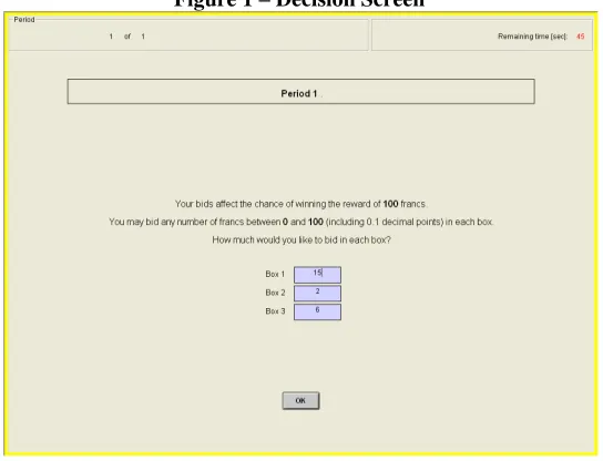
[image:35.612.171.443.205.413.2]Each period you and the other participant in your group will simultaneously make bids (any number, including 0.1 decimal points) in three boxes. Your bid in each box cannot exceed 100 francs. The more you bid, the more likely you are to win a particular box. This will be explained in more detail later. The participant who wins at least two boxes receives the reward of 100 francs. Your total earnings depend on whether you receive the reward or not and how many francs you spent on bidding. An example of your decision screen is shown below in Figure 1:
Figure 1 – Decision Screen
CHANCE OF WINNING A BOX
The more you bid in a particular box, the more likely you are to win that box. The more the other participant bids in the same box, the less likely you are to win that box. Specifically, for each franc you bid in a particular box you will receive one lottery ticket. At the end of each period the computer draws randomly one ticket among all the tickets purchased by you and the other participant in the group. The owner of the drawn ticket wins. Thus, your chance of winning a particular box is given by the number of francs you bid in that box divided by the number of francs you and the other participant bid in that box.
Your chance of
winning a box =
Your Bid in That Box
Your Bid in That Box + The Other Participant’s Bid in That Box In case both participants bid zero in the same box, the computer determines randomly who wins that box. Example: This is an example to illustrate how the computer makes a random draw of lottery tickets. Suppose, in a given round participant 1 bids 10 francs in box 1 and participant 2 bids 20 francs in box 1. Therefore, the computer assigns 10 lottery tickets to participant 1 and 20 lottery tickets to participant 2. Then the computer randomly draws one lottery ticket out of 30 tickets (10 + 20 = 30). As you can see, participant 2 has higher chance, 0.67 = 20/30,whileparticipant 1 has lower chance, 0.33 = 10/30, of winning box 1.
In the sheet attached to these instructions, you will find a probability table. This table will give you some
idea of how your bid and the other participant’s bid affect your chance of winning. For instance, suppose you bid 50
francs and the other participant bid 30 francs then your chance of winning the box is 0.63. Note that as stated before,
your chance of winning increases as your bid increases relative to the other participant’s bid. So if you bid 70 francs
and the other participant is still bidding 30 francs, your chance of winning increases to 0.70. To assist you with calculation of more precise numbers, we will provide you with the Excel calculator in each round. You may use the
calculator to find the chance of winning for any combination of your bid and the other participant’s bid. We will
35
YOUR EARNINGS
Your earnings depend on whether you receive the reward or not and how many francs you spent on bidding. The participant who wins at least two boxes receives the reward of 100 francs. Regardless of who receives the reward, both participants will have to pay their bids in each box. Thus, the period earnings will be calculated in the following way:
Earnings of the participant who won at least two boxes= 100 - (bid in box 1) - (bid in box 2) - (bid in box 3) Earnings of the participant who less than two boxes = 0 - (bid in box 1) - (bid in box 2) - (bid in box 3)
END OF THE PERIOD
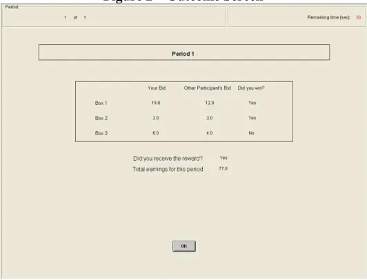
After both participants make their box bids, the computer will make a random draw for each box separately and independently. The random draws made by the computer will decide which boxes you win. The computer will calculate your period earnings based on whether you received the reward or not and how many francs you spent on bidding in each box. Both participants will observe the outcome of the period – your bid in each box, other
participant’s bids in each box, winner of each box, and your earnings from that period, as shown in Figure 2. Once
[image:36.612.173.439.265.468.2]the outcome screen is displayed you should record your results for the period on your Personal Record Sheet under the appropriate heading. You will be randomly re-matched with a different participant at the start of the next period.
Figure 2 – Outcome Screen
END OF THE EXPERIMENT