A projected Lagrangian algorithm for semi infinite programming

by

I. D. Coope and G. A. Watson

*

No. 32 September, 1983

Abstract A globally convergent algorithm is presented for the solution of a wide class of semi-infinite programming

problems. The method is based on the solution of a sequence of equality constrained quadratic programming problems, and usually has a second order convergence rate. Numerical results

illustrating the effectiveness of the method are given.

Keywords Semi-infinite programming, descent algorithm, penalty function, Lagrangian function, global convergence, second order convergence.

1. Introduction

There is currently increasing interest in that class of

opti-mization problems known as semi-infinite programming problems, which

are characterized by a finite number of variables and an infinite

number of constraints. Such problems arise, for example, in air

pollution control, in the solution of weakly singular integral

equations, in probability distributions, etc.: details of these and

other applications may be found in the conference proceedings [ 3 ] ,

(8] and in papers referenced therein. In particular, [ 3] is useful

as a state-of-the-art treatment of the subject area. It is clear

that a large body of theory exists for semi-infinite programming

problems, although with the exception of some special cases, such as

continuous linear Chebyshev approximation, the algorithmic

develop-ment is less far advanced. This is not to say that the provision of

algorithms for general problems has been entirely neglected. A number

of locally convergent methods have been published, mainly based on the

application of Newton's method to first order necessary conditions

for a solution (for example [10] [11]). Suitable initial approximations

can often be obtained through the solution of a discretization of the

original problem, and this has led to the formulation of two (or even

three) phase methods (see, for example,

[6]

and the review paper

[9]).

To our knowledge, the only methods developed so far which claim

to be globally convergent are those given in [13] , [14] (although a

conceptual globally convergent method based on continuation is

suggested in [ 5 ] ) . The algorithm presented in [14] adapts to the

present situation a well-established technique for the globalization

of methods for finite problems, involving the minimization of an

.exact penalty function, and as the numerical results in [14] show,

However, it has two main disadvantages: firstly each iteration

requires the solution of anineq.iality constrained quadratic

programming problem and secondly, fast ultimate convergence

depends on conditions which may well not be satisfied. The

purpose of this paper is to present a modification of that

method which, in particular, overcomes these difficulties.

We begin by introducing the problem to be solved and some

notation. Let X C RN be a c:artesian product of closed intervals

and let g:X x Rn + R, with g twice continuously differentiable

as a function of its parameters. Let f :Rn + R be a twice

continuously differentiable function, and consider the problem:

find~ E Rn to minimize f(~) (1.1)

subject to g (x,a) _{,..., ,...,} ~ 0, Vx E X. _,...,

The algorithm to be developed will be capable of finding a

stationary point of (Ll), defined as follows. We let cp. (a) J ,...., and ~j(~,,~) respectively denote the partial derivatives off

and g with respect to a., j _J

=

1,2, ..• ,n, although the explicit _. dependence on ,?:S and a will sometimes be suppressed when no

confusion can arise.

Definition l. Let,.e* E Rn be feasible in (1.1) and let there

*

exist points x.

"'1.

multipliers A. * I

1.

*

cp . (.e ) ₊ i t

L:

J _i=l

*

* *

with g(x~ ,a) = O, i

=

1,2, •.. ,t and non-negative

"'-1,...,

= 1,2, ..• ,t such that

* *

_*

.:\. tjJ. (x. ,a )

1. J "-'l. ,...,

o,

j = 1,2, ... ,n. (1. 2)

3.

*

The Fritz-John first order necessary conditions for a

*

to solve (1.1) correspond to (1.2) with¢. (a ) replaced by J ,....,

*

-

*

Ao¢j (~ ) , where Ao ;;;:,: 0 (for example [ 1]). I f a first order

*

*

constraint.qualification holds at~ then Ao I 0 and (1.2)

becomes the usual (Kuhn-Tucker) necessary conditions.

A key assumption in the algorithm developed in [14] is that

*

in a neighbourhood of a , the variables ~. representing local

,...., 1.

maxima of the function g(~,,~) can be eliminated from (1.2) by

expressing them as functions of a. For this, we require, in

particular that the implicit function theorem be applicable to

any zero-derivative conditions characterizing these local maxima.

The algorithm in fact requires the more general assumption that

an analogous elimination be possible at all points encountered

in the solution process, and this forces restriction of points

n

~ being considered to a subset B, say, of R at which

appropriate ·conditions hold.

require some further notation.

We now define such a subset and

n In particular, for given~ ER ,

let E(~) denote the set of local maxima of g(~,~) in X which

satisfy <;/" (~, ~ ;;;:,: -

n'

where

n

>

0 is a prescribed constant.

(The role of

n

will become clear subsequently; however it is a

minor one and we will not explicitly show dependence upon it).

Let x EE(~), with cr1, cr2, ••• ,crl the indices of the components

of ~on the boundary of X. Also let 'Vig denote the vector in

Rl

whose components are the partial derivatives of g with respect

" d h . N-l h ' 1

Let v2g enote t e vector in R w ose components are the partia

derivatives of g with respect to the remaining components of x

and let l/22g denote the corresponding (N-l)X(N-l) matrix of

second partial derivatives of g. Then we define B C Rn as the open set of points (assumed non-empty) such that

(1) there are a finite number of points ~ E X such that

(2) at each point of (1) corresponding to a local maximizer of g, l/22g is negative definite and each

component of Vig is non-zero.

The significance of these assumptions is that for ~EB,

appropriate components of each of the p local maximizers x. of

~i

g(·,~) may be regarded locally as differentiable functions of

the parameters ~ through the use of the implicit function

theorem applied to

l/2g(,iS. ,a) = O, i = 1,2, . . . ,p.

1. ,...,,

For any ~ E B, we may therefore define p

f(~) + .2:

1 A.h. (a),

i= 1 1 ,...,,

where

h.(R:,) ₁ = g(x.(a),a), i = 1,2, ... ,p

,...._,J_ ,..._, ~

(1. 3)

the Lagrangian function

(1. 4)

(1. 5)

and the functions x.(a), i = 1,2, ... ,p, are defined by (1.3).

,....,,1,...,,

*

In particular, if a EB, then it is easy to see the relationship

between (1.2) and the usual first order necessary conditions, as the required result carries over directly from the finite

5.

* *

I/ £(a , A. ) = 0 ,

a -... -... ,,..., (1. 6)

*

.where without loss of generality we may assume that t = p(a ) .

~

In addition we mayobtain the corresponding second order conditions in an analogous manner. The relevant results are as follows.

*

*

Theorem 1. Let a EB solve (1.1) and let there exist~ such that (1.6) holds. Then if a certain regularity assumption holds

T 2

* *

s _{,..._,} [I/ _a £(a _{-... -...} ,A. )]s~O _{,..._,}

for all R,: S T l/h , (

a ) =

*

Q f i

=

1 f 2 I • • • f t •

~ ]. ~

*

Theorem 2. Let ~ EB be a feasible point satisfying (1.6) and let

T 2

* *

s [I/ £(a ,A. )]s>o _,,, a -... -.,, ,,...,

T

*

*

for a l l s : s 'Vh. (a)

=

O, i

= 1,2, ... ,t.

Then a is a local ~ ]. ~

solution of (1.1).

The basis of the algorithm developed here is the systematic provision of descent directions for an exact penalty function appropriate to (1.1). Given 8

>

0 such a function may be defined for ~ E B by

(1. 7)

where h.(a), i _{]. ~} = 1,2, ..• ,p is given by (1.5) and (1.3). 'It may be shown by the standard arguments available in the finite case

*

that provided

e

>A,

I i

=

1,2, ... , t then~ EB minimizing

].

In the next section we show how descent directions for P may be calculated at any approximation ~ E B , and

in section 3 we describe a suitable active set strategy, This leads to the detailed statement of the proposed algorithm which is given in section

4.

Numerical results for

an implementation of the algorithm, applied to a number of semi-infinite· programming problems, are presented in section 5.

2. The calculation of descent directions

In the algorithm of

[14],

a descent direction d for P(~) at a point ~ E B is obtained through the solution of the following quadratic programming problem.

Find d E Rn to minimize

£T,S£(~)

+

~£TH£

(2 .1)

subject to h . _{1 ,.._} (a) + _{,.._} d 'ilh. T _{1 _...,} (a) ~ 0 , i = 1 , 2 , •.• , p,,

where H is a given positive definite matrix. It is shown in ~3] that a solution d to (2.1) is a descent direction for P at ~provided that there is a Lagrange multiplier vector

associated with (2.1) which has no component larger than 8. On the other hand, if

£

=

Q

solves (2.1) then examination of the Kuhn-Tucker conditions for (2.1) shows that~ is a stationary point of (1.1) .

A key property possessed by (2.1) is that if H is chosen to be 'i72£(a,A), with a and A approximations to the optimal values, _{,..,.,, ,..,.,, ,..,.,,}

*

7.

the application of Newton's method to the system of equations (1.6)

together with h. (a)= O, i =I ,2, ... ,p. _{]. ,...,} A potential difficulty

* *

however, is that V2£(~,~) may have negative eigenvalues, so that

if H is forced to be positive definite, then the desirable

connection with Newton's method is lost. The intention here is

to maintain that connection by working with an appropriate

equality. constraint quadratic subproblem instead of with (2 .1).

For given a EB, let C be the nXp matrix whose jth colwnn _{,.._,}

is Vh. (a), j = 1,2, •.• ,p and consider.the quadratic programming _{. J ,.._,} problem:

find d E Rn to minimize dT¢ +

~dTHd

,.._, ,.._,

subject to (2.2)

where~.

E

If

has jth component h. (a) and where H is a given

·- J ,.._,

(nXn) symmetric matrix. We assume for the moment that p ~ n.

Let the QR factorization of C (which we will assume to have full rank)

be given by _{C = [ W: Z] [}

_~

_]

( 2. 3)

p n n-p n

where W:R + R, Z:R + R with

[w:z]

orthogonal, and

U:RP +RP is upper triangular. Let

Then if

£1

is chosen to satisfy

T

u .s:!,1 = -,Q, , ( 2. 4) it is clear that the constraints of (2.2) are satisfied and we

are left with an unconstrained problem in the vector £_2.

(2.5)

which has a unique solution provided that the reduced

matrix ZTHZ is non-singular. If the conditions of Theorem 2 are satisfied at a stationary point a*, then ZT [9 2£(a,A)]Z is ,.._, ,.._, ,..,_,

positive definite in a neighbourhood of this point and it is

clear that the choice H = 92£(R:,,~) is appropriate (for some

suitably chosen

2J.

If 92£ is not positive definite (and there is no reason why

it should be) at a stationary point, then the choice H

=

9

2£ + µI

can be used with µ chosen to force positive definiteness of H.

This is the strategy used in

[14]

but it has the disadvantage of

slowing the rate of convergence on some problems. Clearly the

matrix ZTHZ is the one which should be forced to be positive

definite since then the choice H

=

9

2£

+

µI will allow µ

=

0 to be

chosen in a neighbourhood of the solution where the conditions of

Theorem 2 hold. On the other hand, forcing only ZTHZ to be positive definite may cause the solutions to the quadratic programming

subproblems (2.1) or (2.2) to be non-descent directions for the penalty function (1.7) as the following example·illustrates.

(2. 6)

subject to x - a1a2

<

O, x E [0,1].

The extra conditions a1,a2

>

0 have been added to exclude the

lower branch of the hyperbolic constraint; they are not active

'::}.

The set E(~) = {l} is independent of~ in this simple example and

*

t = p(a ) = p(a)

"' "' 1 with the optimal Lagrange multiplier easily

calculated to be A*= 1. The definitions (1.4), (1.5) then give

[

o

-A]

-A

o

which is clearly indefinite.

T

Suppose now that~= (l-E,1-E) and A=~ is the current

* *

2

approximation to (~ ,A ) and choose H = 9 £(~₁A) so that Then the solution to

(2.1)

or

(2.2)

gives

£

= 6(1,l) T,

B

= E +

~E

2

/(l

- E)

which is clearly an excellent direction for 0

<

E

<

1 . . The Lagrange multiplier associated with (2.1) or (2.2) is

1-B/2

>

₁ = A* 1-E

However, the direction~' given by (2.7) is not a descent direction "

for the penalty function (1.7) when

e

=A because the directional derivative, P' (~ ;

£)

=

B

2

>

0. Fortunately i t is always possible (and appropriate) to make £ a descent direction in such cases by increasing the penalty parameter

e

and the following results allow a threshold value to be determined.

Theorem 3. If ZTHZ is positive definite and CTZ = (0) where [c:z] has full rank, then

3a

such that [H + crccT] is positive definite for all 0

>

a .

This is essentially a restatement of the result in [ 4 ;p ·132 ] •

Theorem 4. I f £ solves the quadratic programming problem (2.2) then d also solves:

for any value of o and the Lagrange multipliers of problem (2.8)

"

~(O) say, are related to those of problem (2.2) by the equation

"

~(O)

~(O)

+ 0£. (2.9)

This result is a straightforward application of the Kuhn-Tucker

conditions.

Using Theorems 3 and 4 and Han's result [

7],

we deduce that the solution to problem (2.1) will be a descent direction for the

penalty function (1.7) provided that the parameter

e

satisfies

e~~.(o)

1. i 1,2, ... , p . (2.10)

At points remote from~* it may be necessary to increase 8 in

order to ensure the satisfaction of the inequalities (2.10). Of

-course O will not generally be known so in the algorithm described in section 4 if

,2_,

calculated to solve problem (2.1), is not a descent direction then the current value of

e

must be too small and so it is repeatedly doubled until the directional derivative changes

sign. (For a more detailed description of the overall strategy for

determining a suitable value of

e

see section 4).

3. Active set strategy

In order to obtain a suitable descent direction for the penalty

function (1.7) we have shown that, if the correct active set of

constraints has been identified, it is appropriate to solve

problem (2.2) with the matrix

where )J (~O) is chosen so that ZTHZ is positive definite. Now the

matrix Z depends on the matrix C and this complicates matters when

some of the constraints of problem (2.2) would not be active at the

11.

since it implies that at least one of the Lagrange multipliers of

problem (2.2) is negative, indicating that a;constraint should be

dropped. A further difficulty now arises in that dropping a

constraint causes a column to be deleted from the matrix C, which

in turn results in the matrix Z defined by equation (2.3) having

an extra column. In this case the matrix ZTHZ is increased in size

by one row and column and i t is possible that the current value of

µ may not be large enough to guarantee positive definiteness of

this new ZTHZ matrix. It is, therefore, necessary to consider

increasing µ.when a constraint is deleted. Of course, increasing

µ may mean that the deleted constraint should be reinserted and

this is accounted for in the strategy adopted which essentially

solves a sequence of problems of the form (2.2) but adjusts the

number of equality constraints and the value of µ automatically

until a solution to (2.1) is obtained. Specifically, the active

set method described in [ 4 , pp88-90] is used except that initially,

and whenever a constraint is dropped from the active set, the matrix

H is revised if necessary to make ZTHZ positive definite by

increas-ing µ according to the formula

µ := 4µ + µ ' I

min (3.2)

and by repeatedly applying (3.2) until positive definiteness is

obtained. Initially µ = 0 is always tried, which explains the

need for the extra parameter µ . (

>

0) . min

In a neighbourhood of a*, the solution to equations (2.3) -_,...,..

(2.5) will also usually solve problem (2.1) and the active set strategy is not invoked. If this is not the case, then the solution to

set strategy. The only potential difficulty occurs when p

>

n in which case problem (2.2) has no solution, whereas we assume problem (2.1) always has a solution. This difficulty is also

easily resolved using the active set strategy. All that is required is that some subset of the constraints be used to define_an initial feasible point for problem (2.1). In the algorithm described in the next section we have assumed, for simplicity, that satisfaction of the n most violated constraints (i.e. those with larger values of h.} always gives rise to a feasible point. This is not foolproof

l..

but almost always p ~ n was satisfied for the problems solved in section 5. An exception is in the case of problem 9 which has infinitely many local maxima in the set E(~*) and this caused failure of the algorithm.· (Note, however, that both assumptions

(1) and (2) of section 1 are not satisfied in this case).

4. A projected Lagrangian algorithm

The algorithm described in this section models very closely that described in

[14];

the major difference is due to the method of calculating the descent direction d for the penalty function

(1.7) and this has already been discussed in sections 2 and 3. In order to guarantee descent -of the penalty function P a suitable step lengthy in the direction£ must be determined. As in

[14]

y is chosen as the largest member of the sequence {l,~1~1 • • • }

satisfying

where

T(y,~)~ p I

T(y,~) = P(~,+y£) - P(~)

yP' (~

,2,)

( 4 .1)

.L _) •

and P' (~;~_)

<

0 is the directional derivative of the penalty

function (1.7) at a in the direction d. The value p

=

.0001 was used

I

as in [14] .

In order to calculate H, defined by equations (3.1) and (1.4),

at the start of each iteration i t is necessary to obtain

approximations to the Lagrange multipliers

A.,

i

=

1,2, .•. ,p.

i

Because successive values of p may change at each iteration,

(particularly far from a stationary point) it is not appropriate to

use the Lagrange multipliers of the problem (2.1) as estimates.

Instead,

A

was chosen at the start of each iteration to minimize the

least squares norm of the vector

p

+ .L

1\.;t:_(x. ,a) =

;t_

+ c~

i = i - i ,....,

with any negative components replaced by zeros. This least squares

problem is easily solved, using the QR factorization of the

constraints of ,Problem (2.2), by back substitution in the triangular

system

To complete the definition of H it is necessary to fix a

suitable value for µ . to be used in (3.2). In early numerical min

trials the value µ . = 1 was useo and this usually gave good min

results. However, on some problems when ZTV2£(!:1l)Z was singular

it became clear that ·a smaller value was sometimes more

appropriate particularly when the current approximation a was

far from the solution. Also when ZTV2£(a,\)Z has large negative _{,...., ,....,}

eigenvalues i t makes sense to consider increasing µ Therefore min"

the following rules were used to adjust µ .

nun

through (3.2)) from iteration to iteration.

(and hence µ

(1) I f µ = µ and T

> .

5 and y

min l set µ min

(2) If µ

=

µ . and y ~ ~ set µ .

=

µ . *4.

min min min·

µ . /4

min

The motivation for rule (1) is that if the test is satisfied it indicates that the current value of µ (nece·ssarily greater than zero) may be causing too small a step to be taken in the direction defined by the quadratic programming subproblem. Because T

>

.5 there is reasonable agreement with a linear model and decreasing

µ . by a factor of 4 should cause a corresponding increase in min

the size of d used for the next iteration. In rule (2) the situation suggests that the current step.size,y, has had to be decreased from 1 because the current value of µ is too small and

µ is therefore increased. These rules were found to work very min

well on the range of problems tested and were the ones used to obtain the numerical results of the next section.

15.

to the solution because ~(0) + ~(O) as the solution is approached. This is borne out by the numerical results for problem 14 presented in the next section.

Algorithm summary

(1) Given an approximation~ to a* determine the set E(~) defined in section 1.

(2) Determine a direction d as described in sections 2,3 and increase 8 if necessary so that d is a descent

direction for

P(!,8).

(3) Set R, = ~ + y~ with

Y

chosen to satisfy (4.1). (4) If insufficient accuracy go to step (1).

Step (1) was implemented as in [14]by superimposing a uniform grid on the set X and identifying local maxima on the discrete set of points thus obtained. These discrete local maxima were then refined using a Newton-like iteration. The value

n =

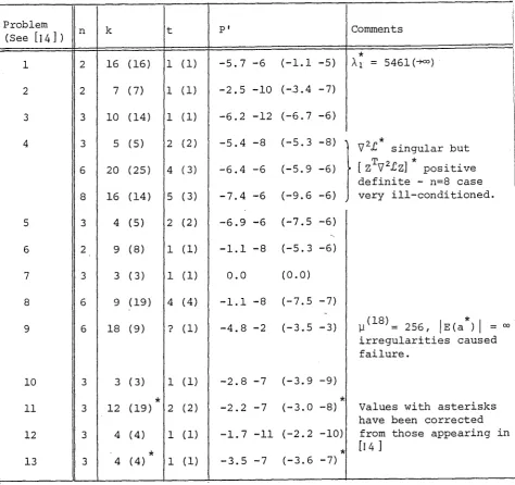
0.5 was used in the definition of the set E(a) given in section 1, in order to _{,.._,,} obtain a valid comparison with the results presented in ~4] and summarized in Table 1.

5. Numerical Results

derivative to a value greater than -.00001, that headed P' gives the

final value of the directional derivative and t gives the final number

of active points. Numbers in brackets correspond to values obtained

by the algorithm in [14] and it can be seen that the present

algorithm compares favourably, There is no significant difference in

the two algorithms on problems 1,2,7,10,12, and 13; of course, it is to

be expected that the two algorithms will give similar results whenever

V2£ remains positive definite throughout the calculation. Significant

improvements were, however, obtained on problems 3,4(n

=

6,8), 8 and 11.

*

Problem 4 is interesting because

V

2

£ ·

is singular and it is worth

considering this problem in detail:

Problem 4

n 3

n

=

6

x

= [ 0, l]

f

g

T Starting point (0,0,0)

f*

=

0.649042

= = n I: i=l tanx a* ,..., T Starting point (O,O,O,O,O,O) ;

a.

l.

i

n

i-1

-

I: a.x

i=l l.

T

=

(0.08910, Q.42305, 1.04526) I

~* = (O.O, 1.02326, -0.24060,

1.22168, -l.38826, 0.94133) I f*

=

0.616085.

n = 8 Starting point: a* for n = 6, to 3 decimal places, with zeros

in the last two components; a*

=

(0.0, 1.00342, -0.06095,

0.75112, -1.40994, 2.65270, -2.311602, 0.03267), f*

=

0.615653.

In each case a* is the point reached by the algorithm when terminated

and f* is the corresponding function value. This problem arises from

l I •

poor choice of basis functions makes the problem severely ill-conditioned

for quite moderate values of n. When n = 6, Table 1 shows that the

earlier algorithm of

(14]

terminated after 25 iterations with a

directional derivative greater than -.00001, and with 3 active points

for the constraint function g. The present algorithm required only 20

iterations and found a solution with 4 active points. Because the

solutions to the two algorithms gave quite different results, the

projected Lagrangian algorithm was rerun using the solution to the n=6

problem, obtained by the algorithm of

(14],

as the starting point. The

new algorithm did not accept this point as a solution but converged once

more to the solution given above. Similar remarks apply to the n=8

case but because this problem is so ill-conditioned it is unlikely that

the solution given above is accurate to more than 3 or 4 significant

figures.

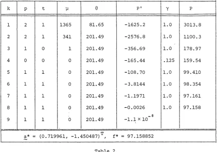
In problem 6, the presence of exponential terms in the constraint

function g(~1~) caused large negative eigenvalues to be present in the

projected Lagrangian Hessian in the early iterations. Initially the

value µ = 1365 was required to make zTV2£z + µI positive definite. This value was reduced to 341 on the ,second iteration and µ = 1 on the third;

thereafter µ

=

0 was acceptable. The detailed progress of the

algorithm on this problem is given in Table 2 and clearly demonstrates

the second order rate of convergence once the correct number of active

points is identified and the projected Lagrangian Hessian becomes

positive definite.

The only problem which caused difficulties for the algorithm was

problem 9. Here the ass1,llllptions of section 1 are not satisfied and

*

1 2 16 (16) 1 ( 1) -5.7 -6 (-1.l -5) )q = 5461 (-+oo)

2 2 7 ( 7) 1 (1) -2.5 -10 (-3.4 -7) 3 3 10 (14) 1 ( 1) -6.2 -12 (-6. 7 -6) 4 3 5 (5) 2 ( 2) -5.4 -8 (-5.3 -8)

}

2

*

V £ singular but 6 20 (25) 4 ( 3) -6.4 -6 (-5. 9 -6) [ TV2£ Z Z

J

*

positive

. .

definite - n=8 case 8 16 (14) 5 ( 3) -7. 4 -6 (-9.6 -6) very ill-conditioned. 5 3 4 (5) 2 (2) -6.9 -6 (-7.5 -6)

~

6 2 9 (8) 1 (1) -1.1 -8 (-5.3 -6) 7 3 3 ( 3) 1 ( 1)

o.o

(0.0) 8 6 9 (19) 4 ( 4) -1.1 -8 (-7. 5 -7)

-µ(18 )= 256,

*

9 6 18 ( 9) ? (1) -4.8 -2 (-3.5 -3)

IE

(a )

I

= 00

irregularities caused failure.

10 3 3 ( 3) 1 ( 1) -2.8 -7 (-3. 9 -9)

*

*

11 3 12 (19) 2 (2) -2.2 -7 (-3.0 -8) Values with asterisks have been corrected 12 3 4 (4) 1 ( 1) -l. 7 -11 (-2.2 -10) from those appearing in

*

*

[I 4 ]

13 3 4 ( 4) 1 (1) -3.5 -7 (-3. 6 -7)

Table 1

[image:19.595.96.571.100.546.2]

Problem 9

19.

X = [ -1 I l] X [ -1 I l]

2

f = -4ai - 3(a4 +as)

g = a1 + azx + a3y + a4x + asxy + a6y2 - 3 - (x2 - y2)2•

Starting point (5,1,1,1,l,l)T ;

~*

= (3,0,0,0,0,0)T, f* -12.

This example has an infinite number of points in E(a*), corresponding

to the line segments of y = .±_x within X. Symmetry in the

components of the starting point caused the algorithm to always generate

T

approximations of the form~= (a,O,O,S,O,S) . At such points the

constraint function g has one maximizing point at the centre of the

region X when S

<

0 and 4 local maximizing points, corresponding to the

four corners of the region X, when

S

>

0. Thus the set E(~) has either one, four or infinitely many members- accordingly as

S

<

O,

S

>

0 or

S

= 0. For

S

<

0 the solution to the subproblem 2.1 always gives a

direction which makes a1 = 3 if y = 1. If the corner constraints

were added to this subproblem then the exact solution would be obtained

in one iteration but unfortunately this can never be the case (unless

S

= 0 when the added complication of jE(~)

I

= 00 _{arises). In practice}

the algorithms switched between using 1 or 4 constraints and in either

case the projected Lagrangian Hessian matrix is singular, and the

choice of µ critically affects the size of the correction at each

iteration. Despite these difficulties the algorithm still made progress

towards the solution and after 18 iterations the approximation

(18) T

a = (3.002, 0.0, 0.0, -.000079, 0.0, -.000079) was obtained. An

error was flagged at iteration 19 because the local maximizer of g had

a numerically singular second derivative matrix, violating assumption 2

of section 1. This was the only problem for which the choice µ

=

0

k p t µ

e

P' y p

1 2 1 1365 81.65 -1625.2 1.0 3013. 8

2 2 1 341 201. 49 -2576.8 1.0 llOO. 3

3 1 0 1 201.49 -356.69 1.0 178.97

4 0 0 0 201. 49 -165.44 .125 159.54

5 1 1 0 201. 49 -108.70 1.0 99.410

6 1 1 0 201. 49 -3.8144 1.0 98.354

7 1 1 0 201. 49 -1.1971 1.0 97.161

8 1 1 0 201. 49 -0.0026 1.0 97.158

_a

9 1 1 0 201. 49 -1.1x10

a*

₌

(0.719961, -1. 450487) TI f*

₌

97.158852

,....,

Table 2

Details for Problem 6

k p t µ

e

P' y p

1 0 0 0 1.0 -5.1 1.0 2.15

2 1 1 0 1.05 +0.05

2.10 -0.22 1.0 2.26

3 1 1 0 1.10 -0.055 1.0 2.2013

4 1 1 0 1.10 -0.0013 1.0 ·2.200000

5 1 1 0 1.10 -8. 2

x

10-7

2:.,*

=

(-.095310, .095310)T ; f*

₌

2.2

Table 3

[image:21.595.100.547.80.393.2] [image:21.595.100.551.91.711.2]

21.

Finally, we introduce a new problem to demonstrate the effect of

a persistent negative eigenvalue in the second derivative matrix of

the Lagrangian function (1.4).

Problem 14

x

= [ 0, l]

f = c2ea1 + ea2

g = x - ea1 + a2

Starting point (0.8, 0.9) T i a* = (in

le

I,

R,n

I

c

I)

T, f* = 2Ic1.

This has essentially the same properties as problem (2.6) but without

the need to include extra positivity constraints. The results of

applying the algorithm to this problem with c

=

1.1 are given in

Table 3. Note that on the second iteration the solution to subproblem

(2.1) gives a non-descent direction for the penalty function, indicated

by the positive directional derivative. However, the matrix

ZT[V 2

£]z

is positive definite so that increasing the penalty parameter

e

temporarily by a factor of two causes the directional derivative to

change sign. The steplength has the value y = l on every iteration

andµ= 0 throughout

e~en

though V2£*

=

L~lcl-1~1]

has one negative

6. Concluding remarks

Th.e algorithm presented in this paper is capable of the

effective solution of a wide class of semi-infinite programming

problems. It is globally convergent under mild assumptions on the

problem, and typically has a second order convergence rate, with

the solution of an equality constrained quadratic progrannning

problem required per iteration. Perhaps the most awkward part of

the method is the computation of the set E(~), which is required

at least once on each iteration. This is of course not a finite

calculation, and must always be a compromise between theory and

practice. It should be emphasised, however, that this is an essential

calculation with any method which aims to provide an accurate

solution to a problem of this semi-infinite type.

It is possible that.far from a stationary point, better progress

can be made for some problems by incorporating a procedure for finding

the solution of a discretization of the original problem. This

remains to be seen, but whether as a method in its own right, or as a

safe and effective second phase for a method of the two-phase variety,

we believe that an algorithm such as the one described in this paper

has an important role to play in the numerical treatment of

semi-infinite programming problems.

Acknowledgement

This research was carried out while the second author was a

23.

References

[ l] Clarke, F. H., A new approach to Lagrange multipliers, Mathematics of Operations Research

l'

165-174 (1976).

[ 2] Charalarnbous, C., A lower bound for the controlling parameter of the exact penalty function, Math. Programming, 17, pp 278-290

(1978).

[ 3] Fiacco, A.

v.

and K. O. Kortanek (eds), Semi-infinite

programming and applications, Proceedings of an international symposium, Springer-Verlag, Berling (1983).

[ 4] Fletcher, R., Practical methods of optimization, vol. II.

Constrained optimization, John Wiley and Sons, Chichester (1981).

[ 5] Gfrerer, H., Guddat, J., Wacker, Hj, and W. Zulehner,

Globalization of locally convergent algorithms for nonlinear optimization problems with constraints, in [3·] , pp 128-137

(1983) .

0

[ 6] Gustafson,

s.

-A., A three-phase algorithm for semi-infinite programs, in [ 3] , pp 138-157 (1983).

[ 7] Han,

s.

P., A globally convergent method for non-linear programming, J. Opt. Theo. Applns, ~, pp 297-309 (1977).

[ 8] Hettich, R. (ed), Semi-infinite programming. Proceedings of a workshop, Springer-Verlag, Berlin (1979).

[ 9] Hettich, R., A review of numerical methods for semi-infinite optimization, in [ 3) , pp 158-178 (1983).

[10] Hettich, R. and W. van Honstede, On quadratically convergent methods for semi-infinite programming, in [8], pp 97-111 (1979).

[11] van Honstede, W., An approximation method for semi-infinite problems, in [ 8], pp 126-136 (1979).

[ 12] Roleff, K., A stable multiple exchange aigorithm for linear semi-infinite programming, in [ 8], pp 83-96 (1979).

[13] Watson, G. A., Globally convergent methods for semi-infinite programming, BIT 21 pp 362-373 (1981).

[14] Watson, G. A., Numerical experiments with globally convergent methods for semi-infinite programming problems, in [3]