Achieving modulated oscillations by feedback control

http://wrap.warwick.ac.uk/

Original citation:

Ge, Tian, Tian, Xiaoying, Kurths, Jürgen, Feng, Jianfeng and Lin, Wei. (2014) Achieving

modulated oscillations by feedback control. Physical Review E (Statistical, Nonlinear,

and Soft Matter Physics), Volume 90 (Number 2). Article number 022909.

Permanent WRAP url:

http://wrap.warwick.ac.uk/64303

Copyright and reuse:

The Warwick Research Archive Portal (WRAP) makes this work by researchers of the

University of Warwick available open access under the following conditions. Copyright ©

and all moral rights to the version of the paper presented here belong to the individual

author(s) and/or other copyright owners. To the extent reasonable and practicable the

material made available in WRAP has been checked for eligibility before being made

available.

Copies of full items can be used for personal research or study, educational, or

not-for-profit purposes without prior permission or charge. Provided that the authors, title and

full bibliographic details are credited, a hyperlink and/or URL is given for the original

metadata page and the content is not changed in any way.

Publisher statement:

© 201

4 American Physical Society

Published version:

http://dx.doi.org/10.1103/PhysRevE.90.022909

A note on versions:

The version presented in WRAP is the published version or, version of record, and may

be cited as it appears here.For more information, please contact the WRAP Team at:

PHYSICAL REVIEW E90, 022909 (2014)

Achieving modulated oscillations by feedback control

Tian Ge,1,2_{Xiaoying Tian,}1_{J¨urgen Kurths,}3,4,5_{Jianfeng Feng,}1,2_{and Wei Lin}1,*

1_{School of Mathematical Sciences, Centre for Computational Systems Biology, Fudan University, Shanghai 200433, China,}

and Key Laboratory of Mathematics for Nonlinear Sciences (Fudan University), Ministry of Education, China

2_{Department of Computer Science, University of Warwick, Coventry CV4 7AL, United Kingdom}

3_{Potsdam Institute for Climate Impact Research, D-14412 Potsdam, Germany}

4_{Department of Physics, Humboldt University of Berlin, D-12489 Berlin, Germany}

5_{Department of Control Theory, Nizhny Novgorod State University, Gagarin Avenue 23, 606950 Nizhny Novgorod, Russia}

(Received 22 November 2013; revised manuscript received 30 May 2014; published 14 August 2014)

In this paper, we develop an approach to achieve either frequency or amplitude modulation of an oscillator merely through feedback control. We present and implement a unified theory of our approach for any finite-dimensional continuous dynamical system that exhibits oscillatory behavior. The approach is illustrated not only for the normal forms of dynamical systems but also for representative biological models, such as the isolated and coupled FitzHugh-Nagumo model. We demonstrate the potential usefulness of our approach to uncover the mechanisms of frequency and amplitude modulations experimentally observed in a wide range of real systems.

DOI:10.1103/PhysRevE.90.022909 PACS number(s): 05.45.−a,02.30.Oz,87.19.lr,89.75.−k

I. INTRODUCTION

Oscillations are omnipresent in the real world, from me-chanics to engineering, from optics to astro- and geophysics, and from economics to social science. In the human body, oscillators are particularly abundant and appear at many different levels, e.g., the oscillatory NFκB signaling pathway in the cell nucleus, the cell cycle, neural oscillations in the central nervous system, and circadian rhythms [1]. The advantages and functional roles of these oscillators have been under active investigation.

In telecommunications, information is encoded and trans-mitted in a carrier wave by varying the instantaneous frequency or strength of the wave, known as frequency modulation (FM) and amplitude modulation (AM), respectively [2]. Recent investigations indicate that FM and AM are not restricted to electronic applications but may be even essential mechanisms of information transmission in a wide range of biological sys-tems. In particular, the period of the cell cycle oscillator ranges from about 10 min in rapidly dividing embryonic cells to tens of hours in somatic cells, while a variation in the amplitude of this oscillation seems neither necessary nor desirable [3]. This is a typical example of FM [4]. In the hippocampus or inferior temporal cortex in the brain, the amplitude of the theta waves (4–8 Hz) increases after learning, while the frequency is approximated invariant. This is a typical example of AM [5]. In spite of the increasing number of phenomenological findings, the common or unique mechanisms that underlie FM and AM in various systems including biological oscillators have remained largely unknown. Initial computational studies suggest that feedbacks play critical roles in generating FM. It is the negative-plus-positive feedback loop that makes some biological oscillators exhibit a widely tunable frequency with a near-constant amplitude [6].

It has been shown recently, in both deterministic and stochastic dynamical models, that feedbacks with or without time delays commonly act as controllers to suppress periodic

*_{[email protected]}

or chaotic oscillations to equilibria or periodic orbits or to synchronize coupled oscillators to a common manifold [7]. However, to the best of our knowledge, few works aim at designing appropriate feedback control to achieve FM and AM in dynamical systems. In this paper, we develop an approach to achieve FM and AM in generic finite-dimensional continuous dynamical systems through feedback control.

II. FREQUENCY AND AMPLITUDE MODULATIONS IN NORMAL FORMS

To begin with, we note that any finite-dimensional con-tinuous dynamical system that exhibits oscillatory behavior through the appearance of an Andronov-Hopf bifurcation can be reduced to a two-dimensional system topologically equivalent to

d dt

x1

x2

=

α −β

β α

x1

x2

−x₁2+x₂2 x1 x2

, (1)

where α and β are real constants [8]. We therefore first investigate FM and AM and illustrate our approach in this normal form. System (1) undergoes a supercritical Andronov-Hopf bifurcation as α passes through zero, where a unique stable periodic orbit bifurcates from the equilibrium x =0. The limit cycle has the amplituder0 =

√

αand the frequency f0=β/2π, respectively. We now introduce to system (1) a

linear feedback control as follows:

x1→x1 x2→x1

x1→x2 x2→x2

=

F11 F12

F21 F22

x1

x2

, (2)

where xi →xj denotes the feedback from xi to xj, and

i,j =1,2,Fij, andi,j =1,2, are the feedback gains. The goal

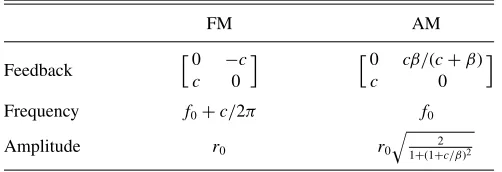
is to design an appropriate linear feedback control by which the controlled system exhibits oscillatory behavior with a modulated amplitude or frequency. This can be easily achieved even if we require that the controlled system undergoes a supercritical Andronov-Hopf bifurcation at the same bifur-cation pointα∗ =0 as in the original system (1) and assume that both self-feedbacks vanish, i.e., F₁₁ =F₂₂=0. Table I

summarizes the designed feedback patterns and the resulting

TABLE I. Frequency and amplitude modulations in the normal form of the Andronov-Hopf bifurcation.

FM AM

Feedback

_{0 −c}

c 0

_{0 cβ/(c+β)}

c 0

Frequency f0+c/2π f0

Amplitude r0 r0

2 1+(1+c/β)2

amplitude and frequency of the controlled system, where we replaceF21 by the parametercfor notational simplicity. The

frequency of the system can be modulated in the range from zero to infinity with an invariant amplitude when a simple antisymmetric feedback is imposed. A positivecincreases the frequency, while a negativecreduces it. The amplitude of the system is less tunable when the autoregulation is constrained at zero. The modulated amplitude is no larger than √2r0,

although the oscillation can be dramatically suppressed when cis sufficiently large.

III. FEEDBACK CONTROL THEORY

To see how the feedback control in TableIis analytically obtained, and, more generally, how FM and AM can be achieved in generic continuous dynamical systems with the constraint on self-feedbacks relaxed, we now present a sketch of our feedback control theory. Full details on the theoretical aspects of our approach are provided in the appendix.

We first note that the investigation of any finite-dimensional and continuous system that undergoes an Andronov-Hopf bifurcation can be reduced to the following generic two-dimensional polynomial system by the center manifold theo-rem [8] and a Taylor expansion at the equilibrium from which the limit cycle bifurcates,

d dt

x1

x2

=

G1(x1,x2;α)

G2(x1,x2;α)

+O(x4), (3)

where Gν(x1,x2;α)= p+q3,p,q0g

ν pq(α)x

p

1x

q

2,ν=1,2,

are polynomials with degrees no larger than 3,p andq are integers, and α is a scalar parameter. We always, without loss of generality, set the equilibrium at the origin by a parameter-dependent coordinate transformation, which indicates that the constants inGν(x1,x2;α),ν=1,2, vanish.

Now we analyze system (3) with the additional linear feedback control (2). The system can then be rewritten as follows:

dx

dt = A(α)x+G(x,α)+O(x

4_{), (4)}

where

A(α)=

g1

10+F11 g011 +F12

g2

10+F21 g012 +F22

(5)

is the Jacobian matrix of the controlled system at the equilibriumx =0, andG(x;α) summarizes all the quadratic and cubic terms.

The key condition for the appearance of an Andronov-Hopf bifurcation at the bifurcation pointα∗is the existence of a pair of complex eigenvalues,λ_±=μ(α)±iω(α), on the imaginary

axis for the Jacobian matrix A(α) atα∗, which is equivalent to (α∗)<0 and tr[A(α∗)]=0, where (α) is the discriminant for the polynomial det [λI−A(α)]. Once these two conditions are satisfied along with the transversality and nondegeneracy conditions, systems with and without linear feedback control can be transformed into their “normal forms” via invertible coordinate and parameter changes when the parameter α is sufficiently close to the bifurcation pointα∗(see the appendix). In the complex domain, the normal form can be written as follows [8]:

dw

dt =λw+ηw

2_{w¯ +O(|w|}4_{), (6)}

where w is a complex variable, ¯w is the conjugate of w, λ=λ(α)=μ(α)+iω(α), andη=η(α) :=χ(α)+iκ(α). If we further require that χ(α)<0, system (4) undergoes a supercritical Andronov-Hopf bifurcation at α=α∗, i.e., a stable limit cycle bifurcates from the equilibrium when α passes through α∗. The amplitude of the invariant curve is approximatelyrF(α)=

√

−μ(α)/χ(α), and the frequency is approximately fF(α)=[ω(α)+κr2F]/2π. Both the

ampli-tude and the frequency are functions ofαand depend on the feedback gains.

As an example, system (1) with feedback control (2) can be converted into the normal form (6), where

λ(α)=α+ i 2

√

− , η(α)≡1 2

−1+F21+β F12−β

<0,

as long as (α)≡(F11−F22)2+4(F12−β)(F21+β)<0,

and tr[A(0)]=F11+F22=0. The amplitude and frequency

of system (1) with feedback control (2) are therefore√−α/η and√− /4π, respectively.

Having obtained the normal forms, it is then straightforward to impose further conditions on the amplitude or the frequency to achieve FM or AM. Specifically, for FM, the amplitude of the limit cycle is invariant with and without linear feedback control. This leads to the following:

r0(α)=rF(α)|Fij=0,i,j=1,2=rF(α). (7) By varying the feedback gainsFij,i,j =1,2, under condition

(7), the amplitude of the oscillator is near constant, while the frequency is tunable. Analogously, for AM, an invariant frequency is required, giving

f0(α)=fF(α)|Fij=0,i,j=1,2=fF(α). (8) Varying the feedback gains Fij, i,j =1,2, under condition

(8), the frequency of the oscillator will remain approximately invariant, while the amplitude can be modulated.

In real applications, optimal feedback control can be searched analytically or numerically in the four-dimensional space {Fij}i,j=1,2, which satisfies Eq. (7) or Eq. (8), while

maximizing a physically or biologically inspired indexJ with certain regularizations on the feedback. For example, the index may be designed as

J =argmaxF{fF/f0−ρF2}, (9)

whereρis a regularization parameter and · 2is the 2-norm of

ACHIEVING MODULATED OSCILLATIONS BY FEEDBACK . . . PHYSICAL REVIEW E90, 022909 (2014)

IV. APPLICATION TO THE ISOLATED FITZHUGH-NAGUMO MODEL

Consider the well-known FitzHugh-Nagumo (FHN) model [9],

dv

dt =v(v−θ)(1−v)−w+I :=p(v)

(10) dw

dt =(v−γ w),

where v mimics the membrane potential of an excitable neuron,wis a recovery variable describing the activation of an outward current, the parameter θ determines the shape of the cubic parabola v(v−θ)(1−v), and γ are non-negative parameters that describe the dynamics of the recovery variablew, andI is the injected current [9]. The FHN model may exhibit a variety of dynamics and can be viewed as a simplification of the Hodgkin-Huxley-type models. The intersection of the v-nullclinep(v)=0 and the w-nullcline w=v/γis the equilibrium of system (10), denoted as (v0,w0).

System (10) undergoes an Andronov-Hopf bifurcation at0=

a0/γif the parameters satisfy 0< a0<1/γor 1/γ < a0<0,

wherea₀=p(v0)= −3v20+2(1+θ)v0−θ. In addition, if

we ensure that

χ(0)= −

1 4

3

2 −

b2 0

1/γ−a0

<0, (11)

whereb₀ =p(v0)/2= −3v0+1+θ, the bifurcation is

su-percritical, i.e., the limit cycle that appears when < ₀ is stable (see the appendix).

We introduce to (10) a linear feedback control as follows:

v →v w→v v→w w→w

=

F₁₁ F₁₂ F21 F22

v−v₀ w−w0

. (12)

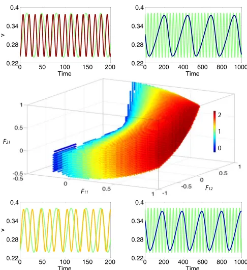
Figure1shows feasible feedback gains that achieve FM in the FHN model with an alteration of the amplitude no greater than 5%. Note that the frequency is widely tunable (approximately 20-fold). The color encodes the index defined in Eq. (9) with ρ=1/4, i.e., a warmer color indicates a larger modulated frequency, penalized by the expense of the feedback control. The time traces of the original and the modulated systems that correspond to two sets of feedback gains are provided in the upper panel. It can be clearly seen that the frequency of the oscillator can either increase or decrease with a near-constant amplitude.

In real-world systems, not all the dynamical equations are accessible for manipulation. One advantage of our approach is that any constraint on the feedback gains can be easily imposed. For example, when the equation of the recovery variablewin the FHN model is not accessible [10],F₂₁ and F22can be fixed at zero, and the frequency of the system is still

widely tunable with an appropriate feedback on the equation of the fast variablevonly (see the bottom panel of Fig.1).

Noise is omnipresent and inevitable in real world. To demonstrate the robustness of our approach with respect to noise perturbations, we consider the following FHN model

0 50 100 150 200

0.22 0.28 0.34 0.4

Time

v

0 200 400 600 800 1000 0.22

0.28 0.34 0.4

Time

0 50 100 150 200

0.22 0.28 0.34 0.4

Time

v

0 200 400 600 800 1000 0.22

0.28 0.34 0.4

Time

2

1

0

F11 F12

F21

FIG. 1. (Color online) Frequency modulation of the FitzHugh-Nagumo model. The model parameters are selected as θ=0.2,

γ =2.5, and I=0.1, which ensure that system (10) undergoes a supercritical Andronov-Hopf bifurcation at 0=a0/γ. Feasible

feedback gains Fij, i,j=1,2, to achieve FM with positive are

numerically searched in the interval [−1,1], with the alteration of the amplitude no greater than 5%. The color encodes the index defined in Eq. (9) with ρ=1/4. The time traces of the original and the modulated systems that correspond to representative points on the surface are provided. The frequency of the system increases with the feedback gainsF11=1.000,F12= −0.450,F21=0.375,

andF22=0.900 (upper left) and decreases with the feedback gains

F11= −0.250,F12=0.950,F21= −0.375, andF22=0.975 (upper

right). When the equation of the recovery variablewis not accessible for manipulation, i.e., F21 and F22 are constrained at zero, the

frequency of the system can also be increased with feedback gains

F11=0.350 and F12= −0.950 (bottom left) and decreased with

feedback gainsF11= −0.250 andF12= −0.850 (bottom right).

with a white noise added to the fast variablev:

dv

dt =v(v−θ)(1−v)−w+I+σ ξ,

(13) dw

dt =(v−γ w),

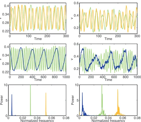
whereσ is the standard deviation of the noise andξ denotes a white noise with zero mean and unit variance. The top and middle panels of Fig.2show the time traces of the perturbed variablevat two different noise levels (σ =0.001 on the left, and σ =0.01 on the right). The model parameters and the feedback control are the same as in the bottom panel of Fig.1. It can be seen that, in the presence of noise, the frequency of the system is still well controlled with the designed feedback. The bottom panels of Fig. 2 present the power spectrum density estimates, with normalized frequencies, of the original and

FIG. 2. (Color online) Frequency modulation of the noise per-turbed FitzHugh-Nagumo model. The top and middle panels show the time traces of the fast variablevat two noise levels,σ=0.001 on the left andσ =0.01 on the right. The bottom panels present the power spectrum density estimates, with normalized frequencies, of the original and controlled systems. The model parameters and the feedback control are the same as in the bottom panel of Fig.1.

controlled systems, which further confirm that the frequency is widely tunable even under noise perturbations.

V. APPLICATION TO A COUPLED FITZHUGH-NAGUMO MODEL

In addition to FM and AM in isolated models, feedback control may play critical roles in networks with coupled oscillators, where FM or AM and synchronization may even be achieved simultaneously.

We illustrate this idea through a coupled FHN model. Specifically, we denote x(t)=[v(t),w(t)] and summarize system (10) into dx/dt=H(x;), where the bifurcation parameteris assigned a proper value to generate oscillatory behavior. We now consider a complex dynamical network described by the following model:

dx(i)

dt =H(x

(i)_;)+Q(i)_{X, (14)}

where i=1,2, . . . ,N is the node index, X(t)= [x(1)(t), . . . ,x(N)(t)] comprises the states of the nodes, and

Q₂N×2N is a coefficient matrix that covers any type of linear

feedback and coupling. Indeed, here we assume that it can be more specifically decomposed as IN×N⊗F2×2+CN×N⊗

I2×2, where ⊗ denotes the Kronecker product, I2×2 is an

identity matrix,F2×2incorporates feedback gains, andCN×N

is the coupling matrix satisfying each row sum to be 1. We note thatFandCare two independent matrices.Fis the feedback gain matrix applied to each two-dimensional system to achieve FM or AM, whileC is a matrix coupling the N oscillators and can be appropriately selected to ensure synchronization in

v

(1

)

v

(

i

)

-0.6 -0.3 0.0 0.3 0.6

FIG. 3. (Color online) The dynamics of N=100 coupled FitzHugh-Nagumo models with linear feedback control. The pa-rameters are selected as θ=0.2, γ =2.5, and I=0.112. is chosen to ensure that each node exhibits oscillatory behavior. Upper panel: The time trace of a single neuron in the network. Lower panel: The dynamics of the 100 neurons in the network. Times 1–600: Q≡0, i.e., each node is an independent FHN neuron with randomly selected initial values. Times 601–900: WhenF11=

0.5000, F12= −2.2024, F21=0.1072, F22= −0.5000, and C is

selected as a compound symmetric matrix in which all diagonal terms are−0.1 and off-diagonal terms are 0.1/99, synchronization in the network is achieved and the resulting synchronous oscillators have an increased frequency. Times 901–1800: When F11= −0.0400,

F12=0.1762,F21= −0.0071,F22=0.0040, andC is selected as

above, synchronization in the network is achieved and the resulting synchronous oscillators have an decreased frequency.

the network. Q(i) in Eq. (14) represents two rows of Qthat correspond to thei-th model.

To simultaneously achieve FM or AM and synchronization, we note that the variational equation of the complex network model on the synchronization manifold reads

dδ(i)

dt =[DH|x(i)+F]δ

(i)_+ν

iδ(i), (15)

where DH_x(i) denotes the Jacobian matrix of H along the

orbit {x(i)_{(t)} and ν}

i is the i-th eigenvalue of the coupling

matrixC. As each row sum ofCequals 1, the matrixCis rank deficient. We therefore assume without loss of generality that ν1=0. The otherνi’s are selected to ensureδ(i)(n) →0, as

n→ ∞, for everyi. This can be validated via numerically cal-culating the Lyapunov exponents of each variational equation transversal to the synchronization manifold.

The upper panel of Fig.3shows the time trace of a single neuron in the network, while the lower panel provides the dynamics of all the 100 neurons. In the first 600 time points,

ACHIEVING MODULATED OSCILLATIONS BY FEEDBACK . . . PHYSICAL REVIEW E90, 022909 (2014)

frequency of the oscillators. This can be seen by noticing much wider stripe patterns compared to the time interval 601–900.

VI. APPLICATION TO THREE-DIMENSIONAL SYSTEMS

Our proposed approach to achieve FM and AM is also applicable to higher-dimensional systems, which resorts to the computation of the center manifold, followed by our generic feedback control theory in two-dimensional systems presented above. As an illustrative example, we consider the following three-dimensional dynamical system:

dx1

dt =(η−1)x1−x2+x1x3, dx2

dt =x1+(η−1)x2+x2x3, (16) dx₃

dt =ηx3−

x₁2+x₂2+x₃2,

where η is a parameter. The system has an equilibrium at (0,0,η), which can be set at the origin via the coordinate trans-formationx1=y1,x2=y2, andx3=y3+η. The transformed

system takes the form

dy1

dt =(2η−1)y1−y2+y1y3, dy2

dt =y1+(2η−1)y2+y2y3, (17) dy3

dt = −ηy3−

y₁2+y2₂+y₃2,

and has the following Jacobian matrix A(η) evaluated at the equilibrium:

A(η)=

⎡

⎣2η1−1 2η−−11 00

0 0 −η

⎤

⎦. (18)

The three eigenvalues of A(η) areλ1,2(η)=2η−1±i, and

λ₃(η)= −η. In particular, whenη=1/2, the equilibrium is not hyperbolic, and the two conjugate eigenvaluesλ₁,2 have

zero real part. By the center manifold theory [8], for each fixed ηwith|η−1/2|sufficiently small, there is a locally defined smooth two-dimensional invariant center manifoldWc

η, which

is tangent at the origin to the generalized eigenspace ofA(η) corresponding to λ₁,2(η). This center manifold Wηc can be

locally represented as a graph of a smooth function,

Wc

η = {(y1,y2,y3) :y3=h(y1,y2)}, (19)

and, due to the tangent property of Wc

η, we write y3=

h(y1,y2)=h20y12+h11y1y2+h02y22+o(y2), where h20,

h11, andh02are functions ofη. By noticing the fact that

dy₃

dt =

∂h(y1,y2)

∂y1

dy₁

dt +

∂h(y1,y2)

∂y2

dy₂

dt , (20)

we find h20=h02 =1/(2−5η) and h11 =0 by expanding

both sides of Eq. (20) and comparing the coefficients of quadratic terms. By the reduction principle [8], for sufficiently small|η−1/2|, system (17) is locally topologically equivalent

near the origin to the system,

dy1

dt =(2η−1)y1−y2− 1 5η−2y1

y₁2+y2₂,

dy2

dt =y1+(2η−1)y2− 1 5η−2y2

y₁2+y2₂, (21)

dy3

dt = −ηy3.

Note that the equation for y3 is uncoupled with y1 andy2

and has an exponentially decaying solution whenη is close to 1/2. Therefore, the stability of system (21) is determined by the equations for y₁ and y₂, i.e., the restriction of the system to its center manifold. Having reduced the system to two dimensions, the standard normal form theory of the Andronov-Hopf bifurcation then follows. In particular, if we introduce a complex variablez=y1+iy2 and transform the

system to its polar form by using the representationz=ρeiφ_,

we obtain dρ

dt =(2η−1)ρ− 1 5η−2ρ

3_+o(ρ3₎

(22) dφ

dt =1.

Since 5η−2>0 for sufficiently small|η−1/2|, the system undergoes a supercritical bifurcation atη=1/2, and a stable limit cycle bifurcates from the equilibrium when η >1/2, with a radius approximately√(2η−1)(5η−2) and a constant frequency 1/2π. The upper panel of Fig. 4 shows an orbit of system (16) with η=1/2+10−3 _{and the initial values}

(0.01,0.01,1.5). Consistent with the theory,x3approaches the

center manifold quickly, on which the orbit converges to the limit cycle.

Higher-dimensional systems offer many more possibilities for the design of feedback control than two-dimensional systems. Here we consider a simple case for illustration. We introduce to the first two components of system (16) an antisymmetric feedback as follows:

x₁ →x₁ x₂→x₁ x₁ →x₂ x₂→x₂

=

0 −β

β 0

x₁ x₂

, (23)

and to the third component a self-feedback,

x3→x3=γ(x3−η), (24)

whereβandγare feedback gains. Repeating the computation that gives Eq. (22), we get the normal form of the controlled system restricted to the center manifold for proper values ofβ andγ,

dρ

dt =(2η−1)ρ− 1 5η−2−γρ

3_+o(ρ3₎

(25) dφ

dt =1+β.

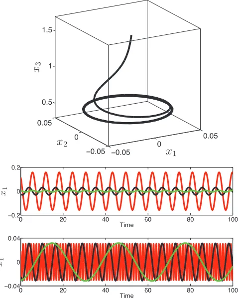
The controlled system then has the same bifurcation point η=1/2 as the original system and has a stable limit cycle with a radius approximately (2η−1)(5η−2−γ), and a frequency (1+β)/2π, whenηis slightly off the critical point. The middle and bottom panels of Fig.4show that the frequency

x

x

x

x1

x1

FIG. 4. (Color online) Frequency and amplitude modulations of an illustrative three-dimensional system. Upper panel: An or-bit of system (16) with η=1/2+10−3 _{and the initial values}

(0.01,0.01,1.5). Middle panel: Amplitude modulation of system (16) with the feedback specified in Eq. (24). Whenη=1/2+10−3_{, the}

amplitude of the original system (black) increases with γ= −12 (red) and decreases withγ=0.48 (green). Bottom panel: Frequency modulation of system (16) with the feedback specified in Eq. (23). Whenη=1/2+10−3_{, the frequency of the original system (black)}

increases withβ=4 (red) and decreases withβ= −0.8 (green).

and amplitude of system (16) can be dramatically modulated whenβandγ are appropriately selected.

VII. DISCUSSION AND FUTURE DIRECTIONS

In this paper, we have presented an approach to design feedback control and modulate the frequency or amplitude of oscillators modeled by generic continuous dynamical systems. In complex network models with coupled oscillators, FM or AM and synchronization can even be achieved simultaneously. The proposed method, when combined with the computation of center manifold, is applicable to FM and AM in higher-dimensional dynamical systems as well.

We note that the normal form theory is accurate when the bifurcation parameter is sufficiently close to the critical point. This somewhat indicates that the above-proposed approach is only suitable for analyzing the behavior of the system near the equilibrium or fixed point, whereas natural systems are believed to operate far from steady states [11]. However, we found that in many cases the feedback control designed near the bifurcation point still can achieve AM and FM when the bifurcation parameter varies in a wide region. For

example, unlike the dynamics presented in Figs. 1 and 2

where the bifurcation parameter is near the critical point (=∗−10−3_{), in the FHN network model presented above,}

is set at ∗−0.1. The system exhibits a much richer dynamics than a regular oscillation only, and the effects of FM are still clearly observed. Hence, our strategies for achieving FM or AM are applicable to oscillations even far from steady states. Having said this, strategies based on global bifurcation theory are also expected for rigorous analysis of the systems not close to the equilibrium or fixed point.

The approach for FM and AM is not restricted to continuous dynamical systems and can be easily applied to discrete dynamical systems that exhibit oscillatory behavior via the appearance of a Neimark-Sacker bifurcation, the counterpart of the Andronov-Hopf bifurcation. Our approach may also be extended to engineering oscillators with nonlinear feedbacks or time delays. Our investigations may invite systematic studies on oscillator control theory and contribute to a general principle to engineer biological oscillators and has the potential to provide a theoretical support to the mechanisms of FM and AM postulated in the literature.

ACKNOWLEDGMENTS

This work was supported by the NNSF of China (Grants No. 11322111 and No. 61273014) and by Talents Programs (Grants No. 10SG02, No. 11QH1400200, and No. NCET-11-0109).

APPENDIX

In this appendix, we provide details of the analytical approach to achieve frequency and amplitude modulations in generic continuous dynamical systems and expatiate on the computational details when applying the theory to the normal form of the Andronov-Hopf bifurcation and the FitzHugh-Nagumo model.

1. Frequency and amplitude modulations in continuous dynamical systems

We note that the investigation of any finite-dimensional system that undergoes an Andronov-Hopf bifurcation can be reduced to the following generic two-dimensional polynomial system by the central manifold theorem [8] and a Taylor expansion at the equilibrium from which the limit cycle bifurcates,

d dt

x1

x2

=

G1(x1,x2;γ)

G2(x1,x2;γ)

+O(x4), (A1)

where Gν(x1,x2;γ)= p₊q3,p,q0gpqν (γ)x p

1x

q

2, ν=1,2,

ACHIEVING MODULATED OSCILLATIONS BY FEEDBACK . . . PHYSICAL REVIEW E90, 022909 (2014)

with an additional linear feedback control,

x1→x1 x2→x1

x₁→x₁ x₂→x₂

=

F11 F12

F₂₁ F₂₂ x1

x₂

,

wherexi →xj denotes the feedback fromxitoxj andi,j =

1,2, Fij, i,j=1,2, are the feedback gains. The system can

then be reorganized as follows:

dx

dt = A(γ)x+G(x,γ)+O(x

4_{), (A2)}

where

A(γ)=

g1

10+F11 g011 +F12

g2₁₀+F21 g012 +F22

is the Jacobian matrix of the controlled system at the equilibriumx=0,

G(x,γ)=Gq(x,γ)+Gc(x,γ).

HereGqdenotes all the quadratic terms as follows:

Gq(x,γ)=

g1

20x21+g111 x1x2+g102x22

g2₂₀x2₁+g₁₁2 x1x2+g202x22

,

Gcsummarizes all the cubic terms,

Gc(x,γ)=

g₃₀1 x₁3+g₂₁1x₁2x2+g121x1x22+g031x23

g₃₀2 x₁3+g₂₁2x₁2x2+g122x1x22+g032x23

,

andgν pq =g

ν

pq(γ), 1p+q 3,p,q 0,ν=1,2, are all

smooth functions ofγ.

The goal is to design an appropriate linear feedback control by which the controlled system undergoes a supercritical Andronov-Hopf bifurcation at the bifurcation point γ∗ and additionally exhibits oscillatory behavior with a desired amplitude or frequency.

The key condition for the appearance of an Andronov-Hopf bifurcation is the existence of a pair of complex eigenvalues on the imaginary axis for the Jacobian matrix A(γ) at the bifurcation pointγ =γ∗, which is equivalent to (γ∗)<0 and tr[A(γ∗)]=0, where (γ) is the discriminant for the polynomial det [λI−A(γ)]. Therefore, we have

(γ∗)=g1₁₀(γ∗)−g₀₁2(γ∗)+F11−F22 2

+4g1₀₁(γ∗)+F12 g102(γ∗)+F21

<0 (A3)

and

tr[A(γ∗)]=g₁₀1(γ∗)+g2₀₁(γ∗)+F₁₁+F₂₂=0. (A4)

Lemma 1. Suppose that gν_pq=gν_pq(γ),1p+q

3,p,q0,ν=1,2, satisfy the transversality and

nondegeneracy conditions atγ =γ∗. Furthermore, conditions Eq. (A3) and Eq. (A4) hold. Then system (A2) undergoes an Andronov-Hopf bifurcation atγ =γ∗.

Suppose that the conditions in Lemma1hold. Then system (A2) can be transformed into its normal form via invertible coordinate and parameter changes. Specifically, Eq. (A3) and Eq. (A4) ensure that, for all sufficiently small|γ −γ∗|, the Jacobian matrixA(γ) has two eigenvalues as follows:

λ_±(γ)=μ(γ)±iω(γ),

whereμ(γ)= 1₂[g1

10(γ)+g201(γ)+F11+F22] withμ(γ∗)=

0 and ω(γ)=1₂√− (γ). Hence, there exists an invertible matrix Psuch that

A(γ)=P J(γ)P−1,

where J(γ)=[μ_ω −_μω] is the Jordan normal form ofA(γ). De-note ξ =ξ(γ)=2[g1

01+F12] and ζ =ζ(γ)=g012 −g110+

F₂₂−F₁₁.Pcan then be selected as

P = 1

ξ

ξ 0

ζ −√−

.

By a coordinate transformation y=P−1x, system (A2) can be transformed into

dy

dt = J(γ)y+K(y,γ)+O(y

4_{), (A5)}

whereK(y,γ)= P−1G(P y,γ)=Kq(y,γ)+Kc(y,γ), with

Kq(y,γ) andKc(y,γ) denoting the quadratic and cubic terms

of K(y,γ), respectively. Note that this transformation leaves the first component of the coordinate unchanged.

Taking into account the following facts:

x₁2 =y₁2,

x1x2 =

y1

ξ [ζ y1− √

− y2],

x₂2 = 1 ξ2

ζ2y₁2− y₂2−2√− ζy1y2

,

and after intensive calculation, we obtain the coefficients in

Kq(y,γ) andKc(y,γ),

Kq(y,γ)=

k₂₀1y₁2+k₁₁1y1y2+k021y22

k2

20y12+k112y1y2+k022y22

,

where kν

pq=kpqν (γ), p+q =2, p,q0, ν=1,2, are

smooth functions ofγ,

k₂₀1 =g₂₀1 +ζ ξg

1 11+

ζ2 ξ2g

1 02,

k₁₁1 = − √

− ξ

g₁₁1 +2ζ ξ g

1 02

, k1₀₂= − ξ2g

1 02,

k₂₀2 = √1 −

ζ g₂₀1 −ξg₂₀2

+√1

−

ζ ξ

ζ g1₁₁−ξg2₁₁+ζ

2

ξ2

ζ g₀₂1 −ξg2₀₂,

k₁₁2 = −1 ξ

ζ g₁₁1 −ξg2₁₁+2ζ ξ

ζ g1₀₂−ξg2₀₂,

k₀₂2 = √

− ξ2

ζ g₀₂1 −ξg₀₂2. (A6)

Kc(y,γ)=

k1₃₀y₁3+k1₂₁y₁2y2+k112y1y22+k031y23

k2

30y13+k221y12y2+k212y1y22+k032y23

,

where k_pqν =k_pqν (γ), p+q =3, p,q0, ν=1,2, are smooth functions ofγ,

k₃₀1 =g1₃₀+ζ ξg

1 21+

ζ2 ξ2g

1 12+

ζ3 ξ3g

1 03,

k₂₁1 = − √

− ξ

g1₂₁+2ζ ξ g

1 12+

3ζ2

ξ2 g 1 03

,

k₁₂1 = − ξ2

g₁₂1 +3ζ ξ g

1 03

, k1₀₃= √

− ξ3 g

1 03,

k₃₀2 = √1 −

ζ g₃₀1 −ξg₃₀2 +ζ ξ

ζ g1₂₁−ξg₂₁2

+√1

−

ζ2

ξ2

ζ g₁₂1 −ξg₁₂2+ζ

3

ξ3

ζ g₀₃1 −ξg₀₃2,

k₂₁2 = −1 ξ

ζ g₂₁1 −ξg₂₁2

−1 ξ 2ζ ξ

ζ g₁₂1 −ξg₁₂2+3ζ

2

ξ2

ζ g₀₃1 −ξg2₀₃,

k₁₂2 = √

− ξ2

ζ g₁₂1 −ξg₁₂2 +3ζ ξ

ζ g₀₃1 −ξg2₀₃,

k₀₃2 = ξ3

ζ g₀₃1 −ξg₀₃2 . (A7)

SinceK(y,γ) satisfies thatK(0,γ)=0for all sufficiently small|γ−γ∗|, by introducing a complex variablez=y1+

iy₂, Eq. (A5) can be transformed into the following complex form:

dz

dt =λz+ l20

2 z

2_+l 11z¯z+

l02

2 z¯

2

+l30

6 z

3₊l21

2 z

2_z¯+l12

2 z¯z

2₊l03

6 z¯

3_+O(|z|4_),

whereλ=λ(γ)=μ(γ)+iω(γ),lpq=lpq(γ),p+q =2,3,

p,q0, are smooth functions ofγ. Specifically,

l20 =

1 2

k1₂₀+k₁₁2 −k₀₂1 +ik₂₀2 −k1₁₁−k₀₂2,

l11 =

1 2

k1₂₀+k₀₂1+ik₂₀2 +k₀₂2 ,

l02 =

1 2

k1₂₀−k₁₁2 −k₀₂1 +ik₂₀2 +k1₁₁−k₀₂2,

l21 =

1 4

3k₃₀1 +k1₁₂+k₂₁2 +3k2₀₃

+i

4

3k₃₀2 −k1₂₁+k₁₂2 −3k₀₃1,

wherekν

pq=kpqν (γ) are specified in Eq. (A6) and Eq. (A7).

Lemma 2. [8]. The equation

dz

dt =λz+ l20

2 z

2_+l 11z¯z+

l02

2 z¯

2

+l30

6 z

3₊l21

2 z

2_z¯+l12

2 z¯z

2₊l03

6 z¯

3_,+O(|z|4_),

whereλ=λ(γ)=μ(γ)+iω(γ),μ(γ∗)=0,ω(γ∗)>0, and lpq=lpq(γ) can be transformed by an invertible

parameter-dependent change of complex coordinate, which is smoothly dependent on the parameter,

z=w+h20

2 w

2_+h 11ww¯ +

h02

2 w¯

2

+h30

6 w

3₊h21

2 w

2_w¯+h12

2 ww¯

2₊h03

6 w¯

3_,

for all sufficiently small|γ−γ∗|, into a map with only one cubic term (theresonant term),

dw

dt =λw+ηw

2_{w¯ +O(|w|}4_),

where

η=η(γ)= l20l11(2λ+λ)¯ 2|λ|2 +

|l₁₁|2

λ + |l₀₂|2

2(2λ−λ)¯ + l₂₁

2 .

Let χ(γ)=Re [η(γ)]. Then the coefficient χ(γ∗) deter-mines the stability of the invariant orbit in system (A2) which undergoes an Andronov-Hopf bifurcation.

Having obtained the normal forms, the stability as well as the amplitude and frequency of the invariant orbit can be extracted, as summarized in the following lemma.

Lemma 3. Suppose that the conditions Eq. (A3), Eq. (A4), and χ(γ∗)<0 are satisfied, along with the nondegenerate condition(γ∗)=0 and the transversality conditionμ(γ∗)= 0. Then system (A2) undergoes a supercritical Andronov-Hopf bifurcation at γ =γ∗. A stable closed invariant orbit bifurcates from the equilibrium when γ passes through γ∗. The direction of this bifurcation is determined by the sign of μ(γ∗). Specifically, the invariant orbit appears forγ > γ∗ if μ(γ∗)>0 and forγ < γ∗ ifμ(γ∗)<0. The radius of the invariant orbit is approximatelyrF(γ)=

√

−μ(γ)/χ(γ), and the frequency is approximatelyfF(γ)=ω(γ)/2π.

To modulate the frequency of the oscillator with an invariant amplitude, all the conditions in Lemma3are required to ensure the appearance of a supercritical Andronov-Hopf bifurcation. Moreover, the amplitude of the stable closed invariant orbit that bifurcates from the equilibrium is invariant with and without linear feedback control. This leads to the following:

rF(γ)|F_ij=0,i,j₌1,2 =rF(γ). (A8)

By varying the feedback gainsFij,i,j =1,2, under Eq. (A8),

the amplitude of the stable closed invariant orbit is approxi-mately invariant while the frequency is tunable.

Similarly, to modulate the amplitude of the oscillator with an invariant frequency, it is required, in addition to all the conditions in Lemma3, that

fF(γ)|Fij=0,i,j=1,2 =fF(γ). (A9)

By varying the feedback gainsFij,i,j =1,2, under Eq. (A9),

the frequency of the stable closed invariant orbit remains approximately invariant while the amplitude can be modulated. In real applications, conditions (A8) and (A9) can either be calculated analytically or validated numerically.

2. Computational details of the normal form

ACHIEVING MODULATED OSCILLATIONS BY FEEDBACK . . . PHYSICAL REVIEW E90, 022909 (2014)

Following the notations in the above section, the controlled system can then be reorganized as

dx

dt =A(α)x+G(x,α), (A10)

where

A(α)=

α+F11 −β+F12

β+F21 α+F22

and

G(x,α)=Gq(x,α)+Gc(x,α),

with g1

30 =g121 =g212 =g032 = −1, and all the other

coeffi-cientsg_pqν =g_pqν (γ),p+q=2,3,p,q0,ν=1,2, vanish. To ensure the existence of an Andronov-Hopf bifurcation at the same bifurcation point as the original system, it is required that the Jacobi matrixA(α) has a pair of complex eigenvalues on the imaginary axis at the critical pointα∗=0, giving

(α)= (α∗)≡(F11−F22)2+4(F12−β)(F21+β)<0

and

tr[A(α∗)]≡F11+F22=0.

Suppose that the above two conditions are satisfied, and|α|is sufficiently close to zero. ThenA(α) has two eigenvalues,

λ_±(α)=μ(α)±iω(α),

whereμ(α)=αandω(α)= 1₂√− (α). Letξ =2(F12−β),

ζ =F₂₂−F₁₁, and

P = 1

ξ

ξ 0

ζ −√−

.

By a coordinate transformationy= P−1x, system (A10) can be transformed into

dy

dt =J(α)y+K(y,α), (A11)

where J(α)=[α_ω −_αω], K(y,α)=P−1G(P y,α)=

Kq(y,α)+Kc(y,α), with

k₂₀1 =k₁₁1 =k₀₂1 =k₂₀2 =k₁₁2 =k₀₂2 =0

and

k1₃₀= −1−ζ

2

ξ2, k 1 21=

2ζ√− ξ2 , k

1

12 =_ξ2, k 1 03=0,

k2₃₀=0, k2₂₁= −1−ζ

2

ξ2, k 2 12=

2ζ√− ξ2 , k

2 03= _ξ2.

By introducing a complex variablez=y1+iy2, system (A11)

can be transformed into the following complex form:

dz

dt =λz+ l20

2 z

2_+l 11z¯z+

l02

2 z¯

2

+l30

6 z

3₊l21

2 z

2_z¯+l12

2 z¯z

2₊l03

6 z¯

2_{, (A12)}

whereλ=λ(α)=α+iω(α),

l20 =l11=l02=0, l21= −1−

ζ2

ξ2 +_ξ2 <0.

Finally, system (A12) can be transformed by an invertible parameter-dependent change of complex coordinate, which is smoothly dependent on the parameter, for sufficiently small |α|, into its normal form with only one cubic term (the resonant term),

dw

dt =λw+ηw

2_w,¯

where

η=η(α)= l21

2 ≡

1 2

−1+F21+β F12−β

<0.

Since χ(α)=Re[η(α)]=η(α)<0, the controlled system (A10) undergoes a supercritical Andronov-Hopf bifurcation atα∗=0. The radius of the limit cycle is

rF(α)=

−α

η,

and the frequency of the invariant orbit is

ω

2π =

1 4π

√ −

= 1

4π

−(F11−F22)2−4(F12−β)(F21+β).

Suppose that both self-feedbacks vanish, i.e.,F11 =F22=

0. To modulate the frequency of the oscillator with an invariant amplitude, we require that

√

α=r0=rF(α)|Fij=0,i,j=1,2=rF(α)=

−α

η,

givingF₁₂= −F₂₁. That is, any feedback control that takes the form [0c −0c] can achieve FM, with a modulated frequency

fF =(β+c)/2π=f0+c/2π.

To modulate the amplitude of the oscillator with an invariant frequency, we require that

β

2π =f0=fF(α)|Fij=0,i,j=1,2 =fF(α)

= 1

4π √

− = 1

2π

(β−F12)(β+F21),

givingF₁₂=βF₂₁/(β+F₂₁). That is, any feedback control that takes the form [0_c cβ/(c₀+β)] can achieve AM, with a modulated amplitude

rF=

2α

1+(1+c/β)2 =r0

2 1+(1+c/β)2.

3. Computational details of the FitzHugh-Nagumo model

Consider the FHN model described by the continuous dynamical system (10). The Jacobi matrix of system (10) at

the equilibrium (v0,w0) is

A0=

a0 −1

−γ

,

where a0 =p(v0)= −3v02+2(1+θ)v0−θ. The

eigenval-ues ofA0are

λ_±=μ()±iω()= a0−γ 2

±

a0−γ

2

2

+2a0−γ 2

1 γ −a0

−a₀

1 γ −a0

.

Therefore, the FitzHugh-Nagumo model undergoes an Andronov-Hopf bifurcation at 0 =a0/γ, if the parameters

satisfy 0< a₀<1/γ or 1/γ < a0<0. At the bifurcation

point, the Jacobi matrixA0has a pair of complex eigenvalues,

±i√a0(1/γ −a0), on the imaginary axis. Following the

procedures described above, system (10) can be transformed into the following complex form:

dz

dt =λz+ b₀

4

1+iμ−a0 ω

(z+z)¯2

−1

8

1+iμ−a0 ω

(z+z)¯3,

where λ=λ()=μ()+iω(), b0=p(v0)/2= −3v0+

1+θ, and it can finally be converted into its normal form,

dw

dt =λw+ηw

2_w,¯

where

η()=b

2 0

8

1 μ2_+ω2

5μ−2(μ−a0)−μ

μ−a₀ ω

2

+b20

8

μ μ2+_9ω2

1+

μ−a0

ω

2

−3

8

−ib

2 0

8 ω

1 μ2_+ω2

1−6μ ω

μ−a0

ω +

μ−a0

ω

2

−ib

2 0

8 ω

3 μ2_+9ω2

1+

μ−a₀

ω

2

−i3 8

μ−a₀

ω ,

and, in particular,

Re[η(0)]= −

1 4

3 2−

b2 0

1/γ −a0

.

Therefore, if we ensure that χ(0)=Re[η(0)]<0, the

Andronov-Hopf bifurcation of the FitzHugh-Nagumo model is supercritical, i.e., the limit cycle that appears when < 0

is stable.

We now introduce to (10) the linear feedback control (12). Let x =[v−v0,w−w0]. The controlled FHN model can

be reorganized as follows: dx

dt =A()x+G(x,), where

A()=

a0+F11 −1+F12

+F21 −γ +F22

and

G(x,)=Gq(x,)+Gc(x,),

withg1₂₀=b0,g130= −1, and all the other coefficientsg

ν pq=

g_pqν (γ),p+q =2,3,p,q0,ν=1,2, vanish. Therefore, we have obtained all the coefficientsgν

pq =gpqν (γ), 1p+q

3,p,q0,ν=1,2, for this polynomial system. We can verify all the conditions required for FM and AM following the results established in this Appendix.

[1] L. Ashall et al., Science 324, 242 (2009); C. Gerard and A. Goldbeter,Proc. Natl. Acad. Sci. USA106,21643(2009); A. Goldbeteret al.,FEBS Lett.586,2955(2012).

[2] J. Proakis and M. Salehi,Digital Communications (McGraw-Hill, New York, 2007).

[3] J. R. Pomereninget al.,Cell122,565(2005). [4] L. Caiet al.,Nature455,485(2008).

[5] A. B. Tortet al.,Proc. Natl. Acad. Sci. USA106,20942(2009); K. M. Kendricket al.,BMC Neurosci.12,55(2011).

[6] T. Y. Tsaiet al.,Science321,126(2008); A. Goldbeter,Nature 420,238(2002).

[7] E. Ott, C. Grebogi, and J. A. Yorke,Phys. Rev. Lett.64,1196 (1990); K. Pyragas,Phys. Lett. A170,421 (1992); ,206,323 (1995); ,Philos. Trans. R. Soc. London, Ser. A364,2309(2006); W. Lin, H. Ma, J. Feng, and G. Chen,Phys. Rev. E82,046214 (2010); J. Luet al.,IEEE Trans. Neural Netw.23,285(2012); Y. Guoet al.,New J. Phys.14,083022(2012); G. Yan, J. Ren, Y.-C. Lai, C. H. Lai, and B. Li,Phys. Rev. Lett.108,218703 (2012); W. Linet al.,Europhy. Lett.102,20003(2013); H. Ma,

W. Lin, and Y.-C. Lai, Phys. Rev. E 87, 050901(R) (2013); J. Sun and A. E. Motter,Phys. Rev. Lett.110,208701(2013); A. Koseska, E. Volkov, and J. Kurths,ibid.111,024103(2013); P. Mencket al., Nat. Phys.9,89(2013); Z. Yuanet al.,Nat. Comm.4,2447(2013).

[8] Y. A. Kuznetsov, Elements of Applied Bifurcation Theory

(Spring-Verlag, New York, 1998).

[9] R. FitzHugh,Biophys. J.1,445(1961); J. Nagumoet al.,Proc. IRE 50, 2061 (1962); C. Rocsoreanu et al., The

FitzHugh-Nagumo Model: Bifurcation and Dynamics(Kluwer Academic,

Boston, 2000).

[10] Although the recovery variable w cannot be experimentally measured in real applications, it can be estimated through the fast variablevby several online estimation methods, such as the adaptive synchronization techniques recently developed in the literature. Therefore, the feedback that uses the signal ofw

can still be realized in our approach.