University of Warwick institutional repository: http://go.warwick.ac.uk/wrap
A Thesis Submitted for the Degree of PhD at the University of Warwick
http://go.warwick.ac.uk/wrap/59757
This thesis is made available online and is protected by original copyright.
Please scroll down to view the document itself.
U N
IV
ER
SITAS WARWICEN
SIS
Evolutionary Methods for the Design of Dispatching Rules
for Complex and Dynamic Scheduling Problems
by
Christoph W. Pickardt
Thesis
Submitted to the University of Warwick
for the degree of
Doctor of Philosophy
Warwick Business School
List of Figures iv
List of Tables vii
Acknowledgements x
Declaration xi
Abstract xii
1 Introduction 1
2 Production Scheduling 5
2.1 Problem Definition and Notation . . . 5
2.1.1 TheαField — Shop Configuration . . . 6
2.1.2 TheβField — Processing Characteristics . . . 6
2.1.3 TheγField — Objective Function . . . 9
2.2 Solution Methods . . . 11
2.2.1 Static Scheduling Problems . . . 11
2.2.2 Dynamic Scheduling Problems . . . 13
3 The Design of Dispatching Rules 17 3.1 Simple Single Stage Problems . . . 17
3.1.1 Minimising Mean Flow Time . . . 18
3.1.2 Minimising Mean Weighted Tardiness . . . 18
3.2 Problems with Sequence-Dependent Setup Times . . . 23
3.2.1 Minimising Mean Flow Time . . . 25
3.2.2 Minimising Mean Weighted Tardiness . . . 28
3.3 Batch Processing Problems with Incompatible Families . . . 30
3.3.1 Minimising Mean Flow Time . . . 31
3.3.2 Minimising Mean Weighted Tardiness . . . 33
3.4 Multi-Stage Problems . . . 36
3.4.1 Minimising Mean Flow Time . . . 36
3.4.2 Minimising Mean Weighted Tardiness . . . 49
4 Methodology 59 4.1 Development of Methods . . . 59
4.2 Evaluation of Methods . . . 60
5 Evolutionary Search for Difficult Problem Instances 64 5.1 Related Work . . . 64
5.2 Algorithm Design . . . 66
5.2.1 Encoding of Solutions . . . 66
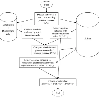
5.2.2 Evaluation . . . 67
5.2.3 Selection . . . 68
5.2.4 Reproduction . . . 69
5.3 Application to a Benchmark Rule from the Literature . . . 70
5.3.1 Scenario Description . . . 70
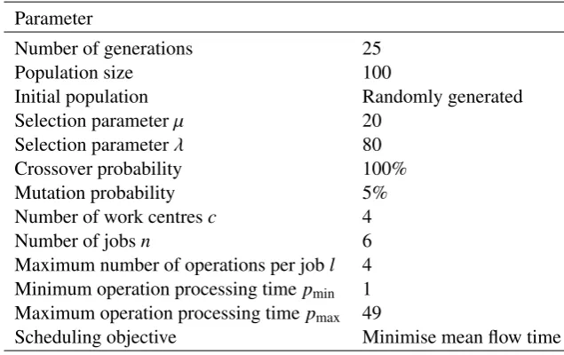
5.3.2 Parameter Setting . . . 71
5.3.3 Analysis of Problem Instances . . . 72
5.3.4 Design of a New Dispatching Rule . . . 77
5.3.5 Applying the Method to the New Rule . . . 79
5.4 Experimental Results . . . 81
5.5 Critical Appraisal and Future Work . . . 83
6 Automatic Rule Generation by Genetic Programming 84 6.1 Related Work . . . 84
6.2 Algorithm Design . . . 87
6.2.1 Encoding of Solutions . . . 87
6.2.2 Evaluation . . . 88
6.2.3 Selection . . . 89
6.2.4 Reproduction . . . 89
6.3 Application to Scheduling Problems from Semiconductor Manufacturing . . 90
6.3.1 Scenario Description . . . 90
6.3.2 Parameter Setting . . . 91
6.4 Experimental Results . . . 94
6.4.1 Minimising Mean Flow Time . . . 95
6.4.2 Minimising Mean Weighted Tardiness . . . 98
6.5 Sensitivity Analysis . . . 102
6.5.2 Due Date Setting . . . 105
6.6 Critical Appraisal and Future Work . . . 107
7 Automatic Generation of Sets of Work Centre-Specific Rules 110 7.1 Related Work . . . 111
7.2 Algorithm Design . . . 113
7.2.1 Encoding of Solutions . . . 113
7.2.2 Evaluation . . . 114
7.2.3 Selection . . . 114
7.2.4 Reproduction . . . 115
7.3 Application to Scheduling Problems from Semiconductor Manufacturing . . 116
7.3.1 Scenario Description . . . 116
7.3.2 Parameter Setting . . . 117
7.4 Experimental Results . . . 118
7.4.1 Minimising Mean Flow Time . . . 119
7.4.2 Minimising Mean Weighted Tardiness . . . 123
7.5 Sensitivity Analysis . . . 127
7.5.1 Arrival Rates . . . 128
7.5.2 Due Date Setting . . . 130
7.6 Critical Appraisal and Future Work . . . 131
8 Conclusion 134
A p-Values of Pairwise Comparisons 136
References 146
List of Dispatching Rules 159
2.1 Example of a setup time matrix for a machine with four possible setups . . . 8
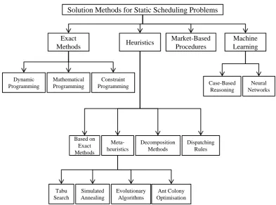
2.2 An overview of solution methods for static scheduling problems . . . 12
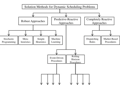
2.3 An overview of solution methods for dynamic scheduling problems . . . 14
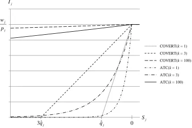
3.1 Influence of the scaling parameterk on the priority index Ij of the COVERT and ATC rules as a function of the slackSjof job j . . . 23
3.2 Classification of setup-oriented dispatching rules . . . 24
3.3 Best practice of setting operation due dates . . . 50
4.1 Simplified diagram of the evolutionary cycle . . . 60
4.2 Moving averages for job flow time for a job shop model from Chapter 5 . . . 61
5.1 Example of the encoding of job shop problem instances asn×2l two-dimen-sional arrays for an instance withn=6 jobs, consisting ofl=4 operations . . 66
5.2 Evaluation of job shop problem instances . . . 68
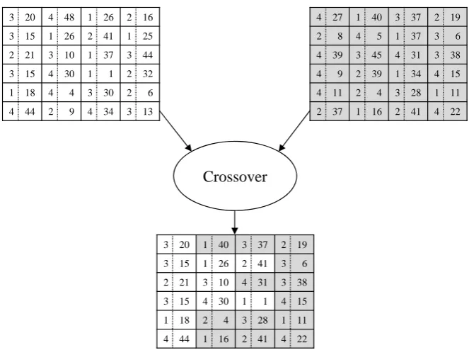
5.3 Example of the crossover operation for job shop problem instances . . . 69
5.4 Example of the mutation operation for job shop problem instances . . . 70
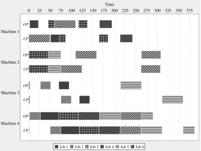
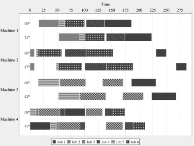
5.5 Problem instance solved ineffectively by PT+WINQ with respect to the mini-mum mean flow time objective — a premature start of a long operation delays arrival of other jobs at the bottleneck machine, which is starving consequently 73 5.6 Problem instance solved ineffectively by PT+WINQ with respect to the min-imum mean flow time objective — prioritisation of a job with long operation delays jobs with short operations and leads to idle times at other machines . . 75
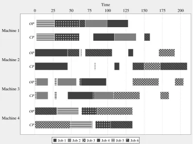
5.7 Problem instance solved ineffectively by PT+WINQ with respect to the mini-mum mean flow time objective — focus of WINQ component on current work contents causes a decision that subsequently leads to unbalanced work con-tents and machine idle times . . . 76
5.8 Problem instance solved ineffectively by IFT−UIT with respect to the
mini-mum mean flow time objective — IFT−UIT delays short jobs by prioritising
a job with a long subsequent operation due to the large amount of idle time it
is estimated to fill in, which turns out to be inaccurate . . . 80
6.1 Example of the encoding of dispatching rules as GP trees . . . 88
6.2 Example of a subtree crossover operation . . . 90
6.3 Example of a subtree mutation operation . . . 90
6.4 Effect of simulation run length, used in the evaluation of individuals, on the performance of the GP hyper-heuristic, measured by the performance of evolved rules . . . 92
6.5 Effect of accounting for warm-up in the evaluation of individuals on the per-formance of the GP hyper-heuristic, measured by the perper-formance of evolved rules . . . 93
6.6 Mean flow time performance of the best evolved rule and the best benchmark rules for the Fab6 shop, subdivided by product type . . . 98
6.7 Mean weighted tardiness performance of the best evolved rule and the best benchmark rules for the Fab4r shop, subdivided by job weight . . . 100
6.8 Mean weighted tardiness performance of the best evolved rule and the best benchmark rules for the Fab6 shop, subdivided by job weight . . . 102
6.9 Performance of the best evolved and the best benchmark rule for the four scheduling problems under varying levels of utilisation . . . 103
6.10 Performance of the best evolved and the best benchmark rule for the two Fab4r problems under varying product mixes . . . 104
6.11 Performance of the best evolved and the best benchmark rule for the two Fab6 problems under varying product mixes . . . 105
6.12 Performance of the best evolved and the best benchmark rule for the twowT problems under varying levels of due date tightness . . . 106
6.13 Performance of the best evolved and the best benchmark rule for the twowT problems under varying levels of due date range . . . 106
7.1 Example of the encoding of dispatching rule sets as one-dimensional arrays for a problem withc=4 work centres . . . 113
7.2 Example of a uniform crossover operation . . . 115
7.3 Example of a uniform mutation operation . . . 116
7.5 Performance of GP rules and rule sets, evolved with and without access to the respective GP rule, for the Fab6 shop with the minimum mean flow time
objective . . . 122
7.6 Mean flow time performance of the best rule set and the best single rule for
the Fab6 shop, subdivided by product type . . . 122
7.7 Performance of GP rules and rule sets, evolved with and without access to
the respective GP rule, for the Fab4r shop with the minimum mean weighted
tardiness objective . . . 124
7.8 Mean weighted tardiness performance of the best rule set and the best single
rule for the Fab4r shop, subdivided by job weight . . . 125
7.9 Performance of GP rules and rule sets, evolved with and without access to
the respective GP rule, for the Fab6 shop with the minimum mean weighted
tardiness objective . . . 126
7.10 Mean weighted tardiness performance of the best rule set and the best single
rule for the Fab6 shop, subdivided by job weight . . . 126
7.11 Performance of the best rule set and the best benchmark rule for the four
scheduling problems under varying levels of utilisation . . . 128
7.12 Performance of the best rule set and the best benchmark rule for the four
scheduling problems under varying product mixes . . . 129
7.13 Performance of the best rule set and the best benchmark rule for the twowT
problems under varying levels of due date tightness . . . 130
7.14 Performance of the best rule set and the best benchmark rule for the twowT
5.1 Parameter setting of the EA to generate difficult-to-solve job shop problem
instances . . . 71
5.2 Determination of job priorities according to the IFT−UIT rule for the problem
instance from Figure 5.6 . . . 78
5.3 Mean flow time performance of newly designed and benchmark rules for ideal
job shops at different utilisation levels . . . 81
5.4 Mean flow time performance of newly designed and benchmark rules for
flow-dominant job shop and flow shop at different utilisation levels . . . 82
6.1 Main features of the two semiconductor manufacturing shops . . . 91
6.2 Parameter setting of the GP hyper-heuristic . . . 94
6.3 Performance of evolved and benchmark rules for the Fab4r shop regarding
mean flow time and mean queueing time . . . 96
6.4 Mean flow time performance of the best evolved rule and the best benchmark
rules for the Fab4r shop, subdivided by product type . . . 96
6.5 Performance of evolved and benchmark rules for the Fab6 shop regarding
mean flow time and mean queueing time . . . 97
6.6 Performance of evolved and benchmark rules for the Fab4r shop regarding
mean weighted tardiness and other due date-related measures . . . 99
6.7 Performance of evolved and benchmark rules for the Fab6 shop regarding
mean weighted tardiness and other due date-related measures . . . 101
6.8 Product mixes generated for the Fab6 shop by means of the random sampling
scheme . . . 105
7.1 Critical work centres of the two semiconductor manufacturing shops . . . 117
7.2 Parameter setting of the rule set hyper-heuristic . . . 118
7.3 Performance of evolved rule sets and benchmark rules for the Fab4r shop
re-garding mean flow time and mean queueing time . . . 119
7.4 Mean flow time performance of the best rule set and the best single rule for
the Fab4r shop, subdivided by product type . . . 121
7.5 Performance of evolved rule sets and benchmark rules for the Fab6 shop
re-garding mean flow time and mean queueing time . . . 121
7.6 Performance of evolved rule sets and benchmark rules for the Fab4r shop
re-garding mean weighted tardiness and other due date-related measures . . . . 123
7.7 Performance of evolved rule sets and benchmark rules for the Fab6 shop
re-garding mean weighted tardiness and other due date-related measures . . . . 124
7.8 Dispatching rules and look-ahead values used at critical work centres as part
I would like to thank both my supervisors, Professor Juergen Branke and Professor Bo Chen,
for their support, especially Juergen Branke for having been so helpful and accessible
through-out the period of my PhD, always showing great interest in my research, which resulted in numerous constructive and fruitful discussions.
I would also like to thank Torsten Hildebrandt and Jens Heger at the BIBA institute at
the University of Bremen, Germany for their contribution to our joint project on Learning and Self-Organisation in Production Planning and Control, and the regular exchange of ideas,
which I have found inspiring and very motivating. In particular, I thank Torsten for his work on the Jasima simulation environment and the technical support he provided with regard to its
extension and its integration with the algorithms developed as part of this thesis.
I am further very grateful to the German Research Council (DFG) for funding the first two
years of my PhD under Grant BR 1592/7-1, and to the Warwick Business School for funding
the third year, which allowed me to conduct this research.
This thesis is submitted to the University of Warwick in support of my application for the
degree of Doctor of Philosophy. It has been composed by myself and has not been submitted
in any previous application for any degree apart from the algorithmic components described in Section 5.2, which were previously developed as part of a thesis submitted for a Master
of Science degree to the Karlsruhe Institute of Technology, Germany. The work presented
(including data generated and data analysis) was carried out by the author.
Parts of this thesis have been published by the author:
• Branke, J. and C. W. Pickardt (2011). Evolutionary search for difficult problem instances
to support the design of job shop dispatching rules. European Journal of Operational
Research212(1), 22–32.
• Pickardt, C. W. and J. Branke (2012). Setup-oriented dispatching rules — a survey.
International Journal of Production Research50(20), 5823–5842.
• Pickardt, C., J. Branke, T. Hildebrandt, J. Heger, and B. Scholz-Reiter (2010).
Generat-ing dispatchGenerat-ing rules for semiconductor manufacturGenerat-ing to minimize weighted tardiness.
In B. Johansson, S. Jain, J. Montoya-Torres, J. Hugan, and E. Y¨ucesan (Eds.),
Proceed-ings of the 2010 Winter Simulation Conference, pp. 2504–2515. Piscataway, NJ: IEEE Press.
• Pickardt, C. W., T. Hildebrandt, J. Branke, J. Heger, and B. Scholz-Reiter (2013).
Evo-lutionary generation of dispatching rule sets for complex dynamic scheduling problems.
International Journal of Production Economics145(1), 67–77.
Three methods, based on Evolutionary Algorithms (EAs), to support and automate the design
of dispatching rules for complex and dynamic scheduling problems are proposed in this thesis.
The first method employs an EA to search for problem instances on which a given dispatch-ing rule performs badly. These instances can then be analysed to reveal weaknesses of the
tested rule, thereby providing guidelines for the design of a better rule. The other two methods
are hyper-heuristics, which employ an EA directly to generate effective dispatching rules. In
particular, one hyper-heuristic is based on a specific type of EA, called Genetic Programming
(GP), and generates a single rule from basic job and machine attributes, while the other
gen-erates a set of work centre-specific rules by selecting a (potentially) different rule for each
work centre from a number of existing rules. Each of the three methods is applied to some
complex and dynamic scheduling problem(s), and the resulting dispatching rules are tested against benchmark rules from the literature. In each case, the benchmark rules are shown to be
outperformed by a rule (set) that results from the application of the respective method, which
demonstrates the effectiveness of the proposed methods.
Introduction
Scheduling is concerned with the allocation of limited resources to tasks over time, with the
basic aim to ensure an effective and efficient use of the available resources. A classic problem
area is the scheduling of manufacturing systems, where machines (the resources) have to be allocated to jobs (the tasks) in a way that the cost of production is minimised. Some of the
costs that are typically affected by a production schedule are the holding costs of process
in-ventory, contractual penalties for late deliveries, setup costs, and the costs of scrap and rework, which illustrates the importance of production scheduling to manufacturers in their endeavour
to become and remain competitive.
In general, scheduling problems can be addressed with a variety of solution methods that
have different strengths and weaknesses (see Pinedo, 2008). However, real-world production
environments tend to be highly complex and dynamic, making the use of some of these
meth-ods impractical. A widely popular approach to solving production scheduling problems in practice are dispatching rules (Pfund et al., 2006), which are simple heuristics that
progres-sively construct solutions by scheduling one operation at a time. More precisely, whenever a
machine is available and there are jobs waiting to be processed on that machine, dispatching rules compute a priority index for each job as a function of some job attributes, e.g. its due
date or the processing time of its imminent operation, and machine attributes, e.g. its current
setup, and schedule only the imminent operation of the job with the highest priority. Dispatch-ing rules thus solve a global problem by makDispatch-ing local schedulDispatch-ing decisions based on local
information, which allows them to be executed very quickly, irrespective of the complexity of
the overall problem. Their ability to take decisions in real-time is particularly advantageous in dealing with dynamic problems as it allows for prompt reactions to sudden changes due
to unexpected events, which can be taken into account as they emerge. Apart from their low computational and information requirements, dispatching rules are further favoured for their
simple and intuitive nature, their ease of implementation and their flexibility to incorporate
domain knowledge and expertise (Aytug et al., 2005).
The main disadvantage of dispatching rules is that, due to their locally restricted horizon,
they cannot assess how a local scheduling decision affects the quality of the global schedule. In
consequence, no rule can outperform all other rules across different shop configurations,
objec-tive functions or operating conditions (Blackstone et al., 1982; Kiran and Smith, 1984; Haupt, 1989; Holthaus and Rajendran, 2000), but they have to be carefully designed for the problem
at hand so that, despite their local horizon, their decisions result in a good global performance.
However, the manual design of effective dispatching rules for complex and dynamic problems
is usually a tedious trial-and-error process, with candidate rules tested in a simulation model
of the considered shop, modified and retested until they meet the demands for actual
imple-mentation, which requires a significant amount of expertise, time and coding-effort (Geiger
et al., 2006). This motivates the development of methods to support and automate the design
of dispatching rules, which is the main concern of this thesis.
Three different methods are proposed in this work, which are each based on an
Evolution-ary Algorithm (EA). The first method employs an EA to search for job shop problem instances
on which a given dispatching rule performs poorly. The idea of this method is to support the
development of dispatching rules by revealing the weaknesses of existing rules. Although sim-ilar methods have been developed by Kosoresow and Johnson (2002) and Julstrom (2009), this
work appears to be the first to apply the idea to dispatching rules, and the area of scheduling in general. Moreover, the proposed EA is designed to search for problem instances where the
poor performance of a tested dispatching rule can be attributed to a single suboptimal decision
it takes, which is a key difference to previous work. The advantage of focussing on single
decision points is that it greatly facilitates the analysis of problem instances and the
identifi-cation of conditions that cause the rule to fail. The effectiveness of the method is assessed by
applying it to a benchmark rule for a well-studied dynamic job shop problem with the objec-tive of minimising mean flow time, where the insights gained from the analysis of the evolved
problem instances are incorporated in the design of two new dispatching rules. The new rules
are then evaluated against the benchmark rule and some other effective rules.
In contrast to the first method, the second method employs an EA directly to search for
effective rules, thereby automating the development process. Such methods that operate on a
search space of heuristics are commonly referred to as hyper-heuristics (Burke et al., 2010). The proposed hyper-heuristic is based on a specific type of EA, called Genetic
Program-ming (GP), and generates a dispatching rule from basic job and machine attributes. Several
researchers have developed similar GP-based hyper-heuristics for various scheduling prob-lems, with promising results (e.g. Atlan et al., 1994; Geiger and Uzsoy, 2008; Jakobovi´c and
Marasovi´c, 2012). However, a shortcoming of these studies is that they predominantly focus
on static problems of small to moderate size, which are likely to be better solved by some global solution method than some dispatching rule. This work investigates the potential of
the developed hyper-heuristic is applied to some dynamic, flexible job shop problems from semiconductor manufacturing with the objectives of minimising mean flow time and mean
weighted tardiness, respectively. These problems feature complex processing characteristics
such as sequence-dependent setup times and batch processing, which make the manual
de-sign of effective dispatching rules very challenging. To assess the effectiveness of the
hyper-heuristic, the evolved dispatching rules are evaluated against some benchmark rules from the
literature, and are further tested for their robustness to changes in the job arrival pattern and due date setting.
The third method is another hyper-heuristic that (automatically) generates a set of work
centre-specific rules by selecting a (potentially) different rule for each work centre from a
number of existing rules. The motivation for this method is that using different dispatching
rules at different work centres has been found to be beneficial for some problems where work
centres vary with respect to their position in the shop (Barrett and Barman, 1986; LaForge and
Barman, 1989; Mahmoodi et al., 1996; Sarper and Henry, 1996; Barman, 1997, 1998) and/or
workload (Raman, Talbot, and Rachamadugu, 1989; Ruben and Mahmoodi, 1998; Bokhorst,
Nomden, and Slomp, 2008). Moreover, similar hyper-heuristics have been developed and
shown to be effective by Baek and Yoon (2002) and Yang et al. (2007) for small problems
with up to ten work centres. This work investigates the potential of EA-based hyper-heuristics to generate sets of work centre-specific rules for complex, dynamic problems that feature a
large set of heterogeneous work centres. The proposed hyper-heuristic is specifically designed
for shops that contain both serial and batch processing work centres, and further extends previ-ously developed hyper-heuristics by optimising the information horizon of each work centre,
i.e. the degree to which jobs that are expected to arrive in the near future are considered
in the decision making. The latter extension is motivated by the observation that it may be beneficial to wait for future jobs at some work centres, e.g. to save a long setup time or to
support the operation of a downstream bottleneck, while it may be counterproductive at
oth-ers, e.g. at highly utilised work centres. The hyper-heuristic is applied to the same problems
as the GP hyper-heuristic, which feature different types of work centres that vary with regard
to their setup requirements, batch processing capacities, number of parallel machines,
work-load and their position in the shop. To assess the effectiveness of the rule set hyper-heuristic,
the evolved rule sets are evaluated against some benchmark rules, including those evolved by
the GP hyper-heuristic, and are further tested for their robustness to changes in the job arrival
pattern and due date setting.
This thesis is organised as follows. Chapter 2 gives a brief introduction to scheduling
problems in production and methods to solve them, and introduces some basic terminology and
notation that is used within the rest of the thesis. Chapter 3 contains a review of dispatching rules, with a focus on promising design concepts for selected problems of interest. Chapter 4
development and evaluation of the three methods, which are subsequently discussed in three separate chapters. In particular, the design and application of the method that employs an EA
to search for problem instances is described in Chapter 5, followed by a presentation of the GP
Production Scheduling
Scheduling problems in production are generally defined by a number of jobs,n, that have to be
processed by a set ofmmachines. The task is to determine a processing order for thenjobs on
each of themmachines, i.e. a schedule, that optimises a given objective function. A scheduling
problem can be either static or dynamic. Staticscheduling problems are deterministic and fully
defined problems with a limited number of jobs, whose attributes are completely known. In
contrast,dynamicproblems are subject to constant change over time due to random, stochastic
events such as new job arrivals or machine breakdowns. This work is primarily concerned
with dynamic scheduling problems, which is motivated by the fact that real-world production
environments are typically dynamic in nature.
This chapter provides a general introduction to scheduling problems and methods to solve
them, with a focus on those type of problems that are most relevant for this work (for a more
ex-tensive discussion on problems and solution techniques in scheduling see Pinedo, 2008). The first section introduces the terminology and the notation used to describe scheduling problems
in this thesis. It also discusses some issues related to the complexity of scheduling problems.
This is followed by another section covering solution methods for static and dynamic schedul-ing problems.
2.1
Problem Definition and Notation
A convenient way to describe a specific scheduling problem is by means of theα|β|γnotation
of Graham et al. (1979), which is adopted herein. The three fields represent the shop
configu-ration, processing characteristics and objective function of the scheduling problem, which are separately discussed in the following.
2.1.1 TheαField — Shop Configuration
A number of shop configurations are commonly described in the scheduling literature. The
simplest configuration is a single machine that is responsible for processing all jobs, which is
denoted by a 1 in theαfield. Pmdenotes aparallel machineenvironment, wheremidentical
machines of the same functionality are available to process a job, whileQmis used to indicate
that the parallel machines differ with respect to their processing speed.Multi-stageproblems,
which are generally NP-hard (Garey et al., 1976), are characterised by jobs that consist of a number of processing steps, or operations, that need to be performed on distinct machines. If
all jobs follow the same route that involves visiting each of the mdistinct machines exactly
once, the shop is called a flow shop, which is denoted by Fm. Hence, every job consists of
exactlymoperations in a flow shop. In the other extreme of an idealjob shop, each job has its
own specified route and may revisit some of themmachines several times while leaving out
others completely. This implies that the number of operations can vary between jobs in a job
shop. In practice, the number of different job routes is often limited by the product portfolio,
which leads to a flow pattern that lies in between the two extremes of the linear flow of a flow
shop and the random pattern of an ideal job shop. Such a shop is referred to as aflow-dominant
job shop herein, and like the ideal job shop, is denoted byJm. Flow shops and job shops are
further called flexible, if they contain at least one work centre that consists of more than one
machine, where awork centreis defined as a set of parallel machines sharing the same input
and output buffer. FFcandF Jcdenote a flexible flow or job shop, respectively, withcwork
centres.
An important characteristic of multi-stage problem is the workload balance among work
centres. In a perfectly balanced shop all work centres are equally utilised, whereutilisation
of a work centre is defined as the fraction of busy time averaged across its machines. On the other hand, an unbalanced shop implies that some work centres have a higher workload than
others. Then, the utilisation of the shop is given by the utilisation of thebottleneck, i.e. the
mostly utilised work centre.
2.1.2 TheβField — Processing Characteristics
The standard assumptions with respect to the processing characteristics of production
schedul-ing problems are that
• a job can be processed by only one machine at at time (no splitting or overlapping),
• a machine can process only one job at a time (no batch processing),
• a started operation must be completed before the respective machine can process another
job (no preemption),
• the processing of jobs is independent of the progress of other jobs (no assembly
opera-tions or precedence constraints),
• processing times are independent of the schedule and cover all activities related to the
execution of an operation (no sequence-dependent setup times),
• machines are the only limiting resource (no lack of operators, tools or material),
• there are no space or time constraints on input and output buffers (no blocking, scrap or
rework),
• all machines are continuously available (no breakdowns or maintenance activities),
• all jobs are available to be scheduled instantly (no dynamic job arrivals).
A problem that fulfils all of the above conditions is typically identified by an emptyβfield.
Otherwise, specific entries are used to indicate certain deviations from these assumptions as
illustrated in the following.
Dynamic Job Arrivals
If jobs arrive at the shop over time, i.e. each job jhas its own specific release daterj, this is
denoted by anrjentry in theβfield. Dynamic job arrivals generally increase the complexity of
scheduling problems, and make some otherwise simple single machine problems become
NP-hard (Lenstra et al., 1977). In reality, perfect information on future jobs and their release dates is often not available, as the job arrival process may depend on external customers placing their
orders. It is thus assumed in this work that future jobs and their characteristics are unknown
until the time of their release to the shop.
Sequence-Dependent Setup Times
Anse f entry in theβfield indicates that machines require to be set up properly to process a
par-ticular job, and that the durations of these setups aresequence-dependent, i.e. they depend on
the current state of the machine, resulting from the previously executed operation. Contrary to
sequence-independent setup times, which can be simply treated as part of the processing time
of an operation, sequence-dependent setup times have to be explicitly modelled and largely increase the complexity of a scheduling problem. This is illustrated by the fact that even the
most trivial single machine problems become NP-hard in the presence of sequence-dependent
setup times (Monma and Potts, 1989; Potts and Kovalyov, 2000).
One way to represent the setup characteristics of a machine is by a so-called setup time
matrix. In practice, the number of different operations a machine can perform will be
be grouped intofamilieswith the implication that changeovers only become necessary when switching from one family of jobs to another. The setup time matrix is a square matrix of
dimension equal to the number of families, where its entries se f specify the time for changing
over from a job belonging to familyeto one belonging to family f. Since no setup is required
between the processing of jobs of the same family, all elements on the main diagonal are equal
to 0 in a setup time matrix. Moreover, setup time matrices normally satisfy the triangle
in-equality, se f +sf g ≥ seg ∀e,f,g(Pinedo, 2008, Chapter 4). The inequality simply states that
the direct transition from one to the other family setup is always the fastest, which is usually
the case in reality. Otherwise, the matrix can be made compliant with the triangle inequality
by substituting the respective entrysegby the lower value ofse f+sf g. Figure 2.1 shows an
ex-ample of a setup time matrix, which satisfies the triangle inequality, for a machine that can be
set up in four different ways. To illustrate, the time for changing over from the setup required
for processing jobs of family 1 to the setup required for jobs of family 3 iss13=2 in this case.
0 3 2 3
5 0 2 3
5 3 0 3
5 3 2 0
Figure 2.1: Example of a setup time matrix for a machine with four possible setups.
A special case of sequence-dependent setup times is the one where all changeovers require
the same amount of time, i.e. all entries of the setup time matrix apart from the zero-diagonal
have the same value. Although setup times are then independent of the family sequence (and have been referred to as being sequence-independent in the literature), they are clearly not
independent of the job sequence as no changeover is required between two jobs of the same
family, and thus have to be modelled as sequence-dependent.
In multi-stage problems, there may be more than one work centre featuring
sequence-dependent setup times. Then, one matrix, which applies to every machine of the respective
work centre, is needed for each of these work centres. Moreover, since the concept of fam-ily membership is generally related to operations and not to jobs, the association of jobs to
families can vary for their different operations in multi-stage problems.
Batch Processing
In contrast toserial processingmachines,batch processing machines can process more than
one job at the same time as a batch. In the literature, a distinction is made between batch
families, a batch can be comprised of jobs with different processing times and of different sizes, and the only constraint regarding the formation of batches is that the total size of a batch
may not exceed the capacity of the machine. The processing time of a batch is then determined
by the maximum of the processing times of the included jobs. The various possibilites to form
batches make these problems difficult to solve, and single machines problems of this type are
already NP-hard, in general (Uzsoy, 1994; Potts and Kovalyov, 2000). On the other hand,
batch processing problems with incompatible families only allow for jobs of the same family to be batched together, which strongly reduces the number of possible batches that can be
formed. In consequence, some common single batch processing machine problems are still
easy to solve if families are incompatible (Uzsoy, 1995).
In the context of batch processing,familiesare defined by jobs that share the same
pro-cessing requirements with regard to machine setup, time and space, and, as in the case of
sequence-dependent setup times, are related to operations in multi-stage problems. Moreover,
the capacity of the machine in terms of the maximum batch sizeBf can vary for different
fami-lies f. In this work, only batch processing problems with incompatible families are considered,
which are identified by aBf entry in theβfield.
2.1.3 TheγField — Objective Function
In practice, the ultimate goal of production scheduling is to minimise the cost of production. However, since cost structures tend to vary widely across companies, general, time-based
objective functions that represent a certain cost component are more commonly used in the
literature. Most of these functions can be classified as being either related to the efficiency of
the shop or its ability to adhere to due dates.
A classic efficiency-related objective of scheduling problems is to minimise themakespan
of jobs, which is the total time required to finish a given set of jobs. In mathematical terms,
the makespan is defined as maxj∈N(Cj), whereNdenotes the set of jobs andCjthe completion
time of job j. Problems with the makespan objective are indicated by aCmaxsymbol in theγ
field. The makespan is an intuitive measure of efficiency for static scheduling problems that
feature a limited and fully defined set of jobs. However, it is generally not a very sensible
criterion for dynamic scheduling problems, in which new jobs arrive continuously.
A more suitable objective for dynamic problems is the minimisation of the mean flow time,
where theflow timeof job jis defined asCj−rj, i.e. the length of time the job spends in the
shop, from the time of its arrival to the time of its completion. The mean flow time is therefore calculated as
1
n
n X
j=1
(Cj−rj)=
1
n
n X
j=1
Cj− 1
n
n X
j=1
rj. (2.1)
of in-process inventory. In Equation (2.1), the last term on the right corresponds to the mean of the job release dates, which are normally not decision variables of a scheduling problem,
but assumed as fixed. Then, they can be taken out of the objective function, and the objective
reduces to the minimisation of the mean completion time. Moreover, the flow time of job jcan
also be written aspj+qj, wherepjindicates its processing time andqjits queueing or waiting
time, which is the reducible component of the flow time. In other words, there is no need to
distinguish between the objectives of minimising average number of jobs in shop, mean (or total) flow time, mean (or total) waiting time and mean (or total) completion time, in this work,
as they all refer to the same objective, which is denoted byC.
Most due date-related objective functions, used to represent costs related to the violation of due dates such as contractual penalties for late deliveries or costs of customer badwill, are some
function of the tardiness of jobs. Thetardinessof job j, denoted byTj, is defined as the
non-negative difference between its completion time and its due datedj, i.e.Tj =max(Cj−dj,0).
Common objectives are the minimisation of the maximum or mean (or total) tardiness of all
jobs, indicated by Tmax and T, respectively, and the proportion (or number) of tardy jobs,
denoted byU. The proportion of tardy jobs can further be seen as one of two components of
the mean tardiness, with the second one being the conditional mean tardiness, which is the
mean tardiness of the tardy jobs and denoted byTcherein. The relationship between the three
measures is given byT =U×Tc.
Pinedo (2008) establishes a complexity hierarchy among the different objectives,
accord-ing to which a schedulaccord-ing problem with the objective of minimisaccord-ing proportion tardy or mean tardiness is generally more complex than the corresponding problem with the maximum
tar-diness objective, which in turn is harder to solve than the respective makespan problem. In
addition, solving a problem for the minimum mean tardiness is at least as hard as to solve it for the minimum mean flow time (Pinedo, 2008, Chapter 2).
In some situations, the costs of holding a job or violating its due date may depend on
the specific job. This is expressed by weighted objective functions, where the contribution of
each job j, e.g. in terms of tardiness or flow time, is multiplied by a weight wj that reflects
its relative importance. The symbolswC andwT indicate the objectives of minimising mean
weighted flow time and mean weighted tardiness, respectively. Clearly, (unequal) job weights increase the complexity of scheduling problems.
The objectives discussed so far are allregular, i.e. the objective function values do not
improve if the completion of a job is delayed. An example of a non-regular objective is the
minimisation of mean earliness, where the earliness of job j, denoted by Ej, is defined as
Ej = max(dj−Cj,0). Such objectives that penalise the earliness of jobs are characteristic of
just-in-time environments, where the aim is to finish jobs dead on time.
To illustrate the notation described in this section, consider a scheduling problem from
het-erogeneous set of work centres, of which some contain multiple machines operating in parallel, and by product-specific routes that involve revisitations. Moreover, some of the machines in
the shop feature sequence-dependent setup times while others are capable of processing
sev-eral jobs simultaneously as a batch (Uzsoy et al., 1992; Pfund et al., 2006). Provided that job arrivals are dynamic and that the objective is to minimise mean weighted tardiness, this
problem is then denoted byF Jc|rj,se f,Bf|wT.
2.2
Solution Methods
In discussing solution methods, a distinction has to be made between methods for static and
dynamic scheduling problems.
2.2.1 Static Scheduling Problems
Static problems are fully defined and, in theory, can be solved to optimality. However, schedul-ing problems in practice are often too complex for exact methods to find the optimum in a
reasonable amount of time, which motivates the use of heuristics and other methods that focus
on delivering a good, but not necessarily optimal solution in a short time. Figure 2.2 presents an overview of methods used to solve static scheduling problems.
Exact solution methods generally involve the formulation of the problem as a (dynamic,
mathematical or constraint) programme that is then solved by a complete and systematic search of the solution space. Many of the more complex scheduling problems can be formulated as
mixed integer programmes (see, e.g. Mason et al., 2005; Pan and Chen, 2005), which are
typically tackled by the well-known branch-and-bound procedure. Exact methods can further be used as heuristics by restricting their search to certain parts of the solution space, or by
setting a limit on the time the algorithm is allowed to run for, after which the best solution found so far is returned.
A different kind of search-based heuristic are the so-called metaheuristics, which start
from initial (randomly generated) solutions that they seek to improve upon by means of local search techniques in combination with mechanisms that allow them to escape local optima
and explore other parts of the solution space. A popular subcategory of metaheuristics are
evolutionary algorithms, which have been widely applied to scheduling (Hart et al., 2005). An alternative heuristic approach to search-based heuristics is to decompose a given
scheduling problem into smaller subproblems that can be solved more easily. These partial
solutions are then combined to yield an overall solution to the original problem. Decomposi-tion methods for static scheduling problems are typically job- or machine-based. An example
of a machine-based decomposition method is the well-known shifting bottleneck heuristic,
Exact
Methods Heuristics
Machine Learning Market-Based
Procedures
Decomposition Methods
Dispatching Rules
Meta-heuristics Based on
Exact Methods Dynamic
Programming
Mathematical Programming
Constraint
Programming Case-Based
Reasoning
Neural Networks
Tabu Search
Simulated Annealing
Evolutionary Algorithms
Solution Methods for Static Scheduling Problems
[image:25.595.123.517.114.405.2]Ant Colony Optimisation
Figure 2.2: An overview of solution methods for static scheduling problems.
A particularly simple type of scheduling heuristic are dispatching rules, which
progres-sively construct solutions by scheduling one operation at a time. Whenever a machine is
available and there are jobs waiting to be processed on that machine, dispatching rules com-pute a priority index for each job (or batch) as a function of some job (or batch) attributes,
e.g. its weight or due date, and machine attributes, e.g. its current setup, and schedule only the imminent operation of the job (or the batch) with the highest priority. Since dispatching
rules lack a global perspective on the problem they tend to produce worse solutions than more
sophisticated heuristics. However, their local horizon allows them to be executed very quickly, irrespective of the complexity of the overall problem.
Another approach that is based on local decision making are market-based procedures,
which model scheduling decisions as a negotiation process between agents associated with jobs and agents representing the machines. Each job agent holds a certain budget, which it
can use to pay for a processing time on the required machine(s). To reserve a time slot for
the imminent operation of a job, the job agent makes a call for bids to which the agents of the machine(s) that can process the operation reply with bids. Each bid consist of a price and
time slot, where the prices are set by the machine agents with the aim to maximise their own
thereby scheduling the operation. A challenge with regard to the application of market-based
procedures is the determination of suitable budgets, as well as effective pricing and acceptance
rules, which are likely to be problem-specific. Toptal and Sabuncuoglu (2010) provide a more
detailed discussion of market-based scheduling procedures.
Finally, static scheduling problems can also be addressed by means of machine learning
algorithms. These algorithms solve problems by inference from good solutions to similar
instances. Hence, they can only be employed in combination with another method or a human expert, which or who generates solutions to example problems that can be used to train the
machine learning algorithm. Some scheduling algorithms based on machine learning can be
found in Pinedo (2008, Chapter 18).
2.2.2 Dynamic Scheduling Problems
Contrary to static problems, dynamic scheduling problems cannot be solved optimally as the optimal solution depends on future uncertain events that occur only after a solution has been
implemented. A key distinctive feature of solution methods for dynamic problems is how they
account for these uncertainties, which can be in a proactive or reactive manner. Figure 2.3
provides an overview of the different methods for dynamic scheduling problems, based on the
surveys by Aytug et al. (2005) and Ouelhadj and Petrovic (2009).
Robust scheduling methods take a proactive approach to uncertainty by generating flexible (or robust) schedules that, up to a certain degree, can accommodate future changes without a
severe deterioration of the objective function value. Measures to increase the robustness of a schedule can include the insertion of idle times at machines that are likely to break down, or
the upkeep of a minimum queue length at the bottleneck work centre to reduce the risk of a
temporarily starving bottleneck due to a breakdown at an upstream machine (Pinedo, 2008, Chapter 18). The drawback of such measures is that they compromise performance to account
for disruptions that do not necessarily occur, e.g. processing capacity may be wasted as a
result of reserving machine time for repair work that turns out to not be required in the end. It is therefore important to have a good understanding of the uncertainties involved in a problem,
their probability of occurrence and their potential impact on the quality of a schedule when
using robust scheduling methods. This knowledge can then be incorporated into the solution method, e.g. into the constraints or objective function of a stochastic mathematical programme
(Kouvelis et al., 2000). However, since predictions regarding future developments become
increasingly inaccurate for longer time horizons, associated with the exponential increase of possible combinations of future events over time, robust scheduling methods are only practical
for problems with relatively short time horizons.
Predictive-reactive methods are two-stage procedures that first generate a so-called predic-tive schedule on the basis of the initial problem data, and then revise and modify this schedule
Completely Reactive Approaches
Market-Based Procedures
Event-Driven Procedures
Dispatching Rules
Rolling Horizon Procedures
Solution Methods for Dynamic Scheduling Problems
Predictive-Reactive Approaches Robust Approaches
Solution Methods for Static Scheduling Problems (see Figure 2.2)
Meta-heuristics
Simple Heuristics Stochastic
Programming
[image:27.595.126.516.106.381.2]Machine Learning
Figure 2.3: An overview of solution methods for dynamic scheduling problems.
time-driven, depending on the mechanism that initiates revisions of the schedule. Event-driven
procedures revise the schedule in response to unexpected events, while time-driven procedures,
commonly referred to as rolling horizon procedures, reoptimise the schedule at regular inter-vals. Concerning the generation of the predictive and revised schedules, any of the solution
methods for static scheduling problems, shown in Figure 2.2, can be used in principle, where the suitability of a method for a given problem generally depends on the nature of the present
uncertainties in terms of their disruptive power and the available time to react. In the case that
the only random events concern the arrival of new jobs that hardly affect the quality of the
current schedule, a rolling horizon procedure, which periodically applies a computationally
expensive branch-and-bound algorithm, may be the method of choice (see, e.g. Ovacik and
Uzsoy, 1994). On the other hand, a problem in which unexpected machine breakdowns can cause sudden and serious disruptions may require for an event-driven method that, in case of
a breakdown, quickly restores feasibility of the schedule by means of a simple heuristic (see,
e.g. Yamamoto and Nof, 1985). In practice, hybrid methods that generally follow a periodic reoptimisation but are able to react flexibly, if the disruption caused by a particular event is
Completely reactive methods are characterised by making scheduling decisions in real-time, immediately before they are implemented, thereby renouncing to plan into the future.
The advantage of this approach is that changes due to random events are taken into account
as they emerge, which allows for prompt reactions. However, in order to be able to schedule in real-time, reactive methods have to rely on procedures with low computational and
infor-mation requirements such as dispatching rules or simple agent negotiation protocols, which
take scheduling decisions on the basis of a locally restricted information horizon with little consideration of the overall problem structure.
In general, there is broad agreement in the literature that the higher the dynamics of a
scheduling problem, the better completely reactive methods fare in comparison to predictive-reactive methods (Aytug et al., 2005). Clearly, a globally optimised schedule becomes obsolete
more quickly if the frequency and impact of random events is high, up to a point where the
assumptions underlying the schedule become invalid only moments after the very first part
of the schedule has been implemented. Then, the global solution method effectively solves
the wrong problem(s) and thus may well lead to poorer scheduling decisions than a locally
restricted method that does not plan into the future at all.
The use of a predictive-reactive approach based on global solution methods may also
be-come impractical if the given scheduling problem is too complex to permit the generation of good global schedules in a reasonable amount of time (Ouelhadj and Petrovic, 2009). The
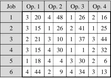
limits of global optimisation methods is impressively demonstrated by a study by Mason et al.
(2005), who apply the well-known CPLEX solver to a mixed integer programming
formula-tion of theF Jc|rj,se f,Bf|wT problem. CPLEX is shown to be unable to find, within six hours
of CPU time, a feasible, let alone the optimal solution to problem instances with only five
machines and nine jobs, consisting of six operations each. In contrast, real-world problems from semiconductor manufacturing, which feature similar processing characteristics (see
Sec-tion 2.1), typically require thousands of operaSec-tions to be scheduled on hundreds of machines
at a time, making the generation of good global schedules extremely difficult.
In summary, a variety of methods exist for solving scheduling problems, which further
can be employed as hybrid methods in various combinations. Solution methods for dynamic
problems can be classified as robust, predictive-reactive and completely reactive. Robust meth-ods try to accommodate uncertainty by anticipating future events, and by themselves are thus
only practical for problems with relatively short time horizons. On the other hand,
schedul-ing problems can be too dynamic or complex for predictive-reactive methods to be effective,
which motivates the use of completely reactive methods with their local decision making.
Completely reactive methods can be based either on dispatching rules or market-based
procedures. While the latter have to be properly configured for the problem at hand, which is generally not easy, dispatching rules are known for their simple and intuitive nature, their
(Aytug et al., 2005). These factors, together with the low computational and information requirements of dispatching rules, explain their wide usage in practice (Pfund et al., 2006) and
the ongoing research on the development and evaluation of dispatching rules. The following
The Design of Dispatching Rules
Since dispatching rules are simple heuristics with a locally restricted information horizon, it
is obvious that no rule can outperform all other rules across different shop configurations,
objective functions or operating conditions (Blackstone et al., 1982; Kiran and Smith, 1984; Haupt, 1989; Holthaus and Rajendran, 2000). Hence, dispatching rules should be generally
designed for the problem at hand, and their priority indices should incorporate attributes that
are specifically relevant with respect to the given problem. In consequence, many different
dispatching rules have been developed over the last few decades (for extensive surveys see,
e.g. Panwalkar and Iskander, 1977; Blackstone et al., 1982; Haupt, 1989).
The aim of this chapter is to highlight the issues in developing effective dispatching rules
as well as to identify the most promising design concepts from the literature for selected
prob-lems of interest. In particular, the scope of the review is on rules designed for scheduling
problems with the objective to minimise mean flow time or mean (weighted) tardiness, where
problems are covered in increasing degree of their difficulty. Thus, the first section presents
rules for simple single stage problems, which provide the basis for the development of more
sophisticated rules for problems with sequence-dependent setup times, batch processing prob-lems or multi-stage probprob-lems, discussed in the three subsequent sections. Throughout this
thesis, priority indices are defined so that a higher indexIjcorresponds to a higher priority of
the job.
3.1
Simple Single Stage Problems
The design of effective dispatching rules for scheduling problems with a single processing
stage or work centre and without complex characteristics such as sequence-dependent setup
times is comparatively easy, and similar principals apply with regard to single machine and parallel machine problems.
3.1.1 Minimising Mean Flow Time
The 1||CandPm||Cproblems are both optimally solved by the Shortest Processing Time (SPT)
rule, according to which jobs are scheduled in non-decreasing order of their processing times
(Smith, 1956; Pinedo, 2008, Chapters 3 and 5). Thus, the priority index of SPT for job jcan
be simply defined as
ISPTj =−pj. (3.1)
The application of the SPT rule is further the best one can do for the analogous problems with
dynamic job arrivals without information on future jobs, which are assumed to be unknown in
this work.
3.1.2 Minimising Mean Weighted Tardiness
Du and Leung (1990) show that the easiest type of this problem category, namely the 1||T
problem, is already NP-hard. Hence, a dispatching rule (polynomial time algorithm) that
optimally solves the 1||wT orPm||wT problem is not known, and its existence is very unlikely.
However, there are two extreme cases that can be solved by a simple dispatching rule.
First, consider the case in which it is impossible to finish any job on time. The mean
weighted tardiness can then be rewritten as
1
n
n X
j=1
wjTj = 1
n
n X
j=1
wj(Cj−dj)= 1
n
n X
j=1
wjCj− 1
n
n X
j=1
wjdj, (3.2)
where the last term of the expression on the right is a constant and independent of the schedule. Hence, the objective of minimising mean weighted tardiness becomes the same as minimising
mean weighted completion time in this case. The 1||wC problem, in turn, is optimally solved
by the Weighted Shortest Processing Time (WSPT) rule by Smith (1956), which also yields
close to optimal solutions to the Pm||wC problem (Pinedo, 2008, Chapters 3 and 5). The
priority index of job jwith WSPT is the ratio of its weight to its processing time, i.e.
IWSPTj = wj pj
. (3.3)
The other extreme case is the one where it is possible to finish every job on time. Then,
an algorithm that minimises the maximum tardiness will produce a solution with a maximum
tardiness of 0, which is obviously also optimal with respect to the mean weighted tardiness
criterion. The 1||Tmaxproblem is optimally solved by the Earliest Due Date (EDD) rule, which
simply schedules jobs in non-decreasing order of their due dates (Jackson, 1955; Pinedo, 2008,
IEDDj =−dj (3.4) or
IEDDj =−(dj−t), (3.5)
wheretrefers to the current time.
Both priority indices represent the same rule as the current time is the same for all jobs and
hence does not affect the ranking of priorities. However, as soon as EDD is integrated with
other rules into so-called composite dispatching rules, the formulation of its priority index
does become important. If the absolute due date from Equation (3.4) is integrated with other
job attributes, their relative proportions, and hence the behaviour of the rule, may change
over time. To illustrate, a dispatching rule with a priority index Ij = −max(10pj,dj) might
operate like SPT in the beginning and then switch to EDD dispatching as time passes and due dates take on substantially larger values than the processing times, which do not change with
time. Clearly, such a time-dependent switch is generally not desired and can be avoided by
relating due dates to the current time as in Equation (3.5), before integrating them with other
attributes. In fact, the termdj−t, which is called theremaining allowanceof job j, appears in
many effective due date-oriented rules, as shown in the following.
The analytical result that EDD and WSPT each lead to an optimal solution to the 1||wT
problem under opposed extreme conditions seems to carry over to the problem with dynamic
job arrivals to some extent. Baker and Bertrand (1982) apply (W)SPT and EDD to the 1|rj|T
problem, and find that SPT clearly outperforms EDD under tight due date levels, while the latter is the better rule if due dates are loose. As a consequence, they propose the Modified
Due Date (MDD) rule, which behaves like SPT or EDD in the respective extreme conditions
and presents a compromise for intermediate tightness settings. Its priority index is defined as
IMDDj =−max(t+pj,dj), (3.6)
i.e. the priority of a job is determined by the maximum of its earliest possible completion time and its due date. Kanet and Li (2004) reformulate the priority index of MDD, by substracting
t, to
IMDDj =−max(pj,dj−t). (3.7)
The terms of earliest possible completion time and due date in the original formulation are
thus replaced by the processing time and remaining allowance of a job, the priority indices of
SPT and EDD. Baker and Bertrand (1982) test MDD against SPT and EDD on the 1|rj|T
prob-lem with various levels of shop utilisation and due date tightness, as well as different due date
conditions. The dominance of MDD over EDD and SPT for the 1|rj|T problem is confirmed
by Moser and Engell (1992a) for different levels of utilisation and due date tightness.
Kanet and Li (2004) extend the MDD rule to the Weighted Modified Due Date (WMDD)
rule to account for unequal job weights. They formulate this extension on the basis of the MDD index from Equation (3.7) and define its priority index as
IWMDDj =− 1
wj
(max(pj,dj−t)). (3.8)
Their decision not to base the WMDD rule on the original MDD index from Equation (3.6)
is motivated by the aim to create a rule that reverts to WSPT behaviour when due dates are very tight. This is achieved by their WMDD formulation, but not by an extension that is
based on the priority index from Equation (3.6), which would prioritise jobs in non-increasing
order of the term (t+ pj)/wj in tight due date settings. They also mention some preliminary
simulation experiments showing this alternative rule to be inferior, which supports the earlier
notion that it is more sensible to use the remaining allowance than absolute due dates within
composite rules. Kanet and Li compare the performance of WMDD for the 1||wT and the
1|rj|wT problem to that of various other rules, and conclude that WMDD is one of the most
effective rules tested.
In trying to minimise mean (weighted) tardiness, it is important to discriminate jobs on the basis of how urgent they are with respect to their individual due dates. One such measure
for the urgency of a job is thecritical ratio, which is generally defined as the fraction of the
remaining allowance of a job to the remaining time required for its completion (Blackstone et al., 1982; Baker, 1984). Thus, the more urgent a job, the smaller its critical ratio, with
a ratio lower than 1 indicating that the job is too far behind schedule to finish on time. By
prioritising jobs in non-decreasing order of their critical ratio, the Critical Ratio (CR) rule aims to minimise mean tardiness by processing the more urgent jobs first. In the context of
simple single stage problems, the remaining time required for the completion of a job is just its processing time and the priority index of CR is thus given by
ICRj =−dj−t
pj
. (3.9)
A general issue with rules that are based on a ratio as priority index is that their behaviour can change as a result of a change of sign in either the numerator or denominator. To illustrate,
the CR rule generally gives priority to jobs that require more time before they are completed.
However, when some jobs have missed their due dates (at which point their priority indices become positive) the rule tends to prioritise the shorter among those late jobs. This anomaly
has been criticised as one of the main drawbacks of ratio type rules, and efforts have been made
prioritisation of short jobs when some jobs are late can be considered a beneficial adaptation to the changing conditions (Vepsalainen and Morton, 1987), as scheduling the tardy jobs first, in
non-decreasing order of their processing times, is actually a sensible strategy to reduce mean
tardiness. The anomaly, however, does mean that the incorporation of weights into the priority index of the CR rule is not trivial. The aim of a weighted variant of CR should be to always
assign a higher priority to jobs with larger weights, no matter whether jobs are late or not. In
practice, a hierarchical rule is often used that prioritises jobs in non-increasing order of their weights, and uses the CR priority index to break ties (Pfund et al., 2006).
Another popular measure for the urgency of a job is the difference (rather than the fraction)
of the remaining allowance and the remaining time required for its completion, commonly
known as theslack (Baker, 1984). For simple single stage problems, the slackSj of job jis
calculated as
Sj =dj−t−pj. (3.10)
The direct use of the slack as a priority index in form of the Minimum Slack (MS) rule, which
schedules jobs in non-decreasing order of their slack, is generally not recommended. This is due to the inherent ‘anti-SPT’ logic (Baker, 1984; Vepsalainen and Morton, 1987), i.e. the
tendency to prioritise longer jobs and thereby counteracting SPT, which can lead to a very poor
performance in conditions of tight due dates. However, the slack is a recurring component of
many of the more effective due date-oriented rules, e.g. the priority index of the CR rule can
be reformulated as
ICRj =−dj−t
pj − pj
pj = −Sj
pj
, (3.11)
sincepj/pjis a constant and constants do not affect the relative priority of jobs. The expression
on the right in Equation (3.11) is the priority index of the Slack per Remaining Processing Time
(S/RPT) rule, which is thus equivalent to CR (Kutanoglu and Sabuncuoglu, 1999). Moreover,
there is an alternative slack-based formulation of the WMDD rule, i.e.
IWMDDj =
−dj−t
wj
ifSj≥0,
−pj
wj
otherwise,
(3.12)
in which the slack can be seen to trigger a switch from a weighted version of EDD to WSPT when jobs become time-critical (Baker and Bertrand, 1982).
Another promising approach, in which the slack plays an important role, are dispatching
rules that determine the priority of a job by estimating the cost of delaying it by one unit of time. Clearly, for a job that is behind schedule, the penalty for delaying it for a further time
unit in terms of increased weighted tardiness is equal to the weight of the job. However, if a job
the cost of taking that decision can only be estimated, e.g. by taking into account the slack of the job. Two popular examples of this type of rule are the Cost Over Time (COVERT) and the
Apparent Tardiness Cost (ATC) rule. While both rules are similar in that they prioritise jobs in
non-increasing order of the ratio of its estimated delay cost to its (imminent) processing time,
they differ with respect to how they estimate the delay cost.
The priority index of the COVERT rule, developed by Carroll (1965), is given by
ICOVERTj = wj pj
max 1− max(Sj,0)
kqˆj ,0
!!
, (3.13)
where ˆqjindicates the estimated queueing time of job jandkis a scaling parameter. As can be
seen from Equation (3.13), the estimated delay cost (and the priority index) of a job decreases
linearly in the amount of its slack, up to a point where the slack exceedskqˆj. Such jobs are
considered to have excessive slack so that a delay does not cause any increase of weighted tardiness, and their estimated delay cost is thus 0. Obviously, the performance of COVERT is
affected to some extent by the method used to determine the queueing times ˆqj. Carroll (1965)
runs a preliminary simulation experiment with the First Come First Served (FCFS) rule to obtain an estimate for the queueing times. Other possible options are to use recently observed
queueing times or initial allowances (Russell et al., 1987).
The ATC rule originates from a paper by Morton and Rachamadugu (1982), and its priority index is defined as
IATCj = wj pj
exp −max(Sj,0)
k p
!
. (3.14)
The main difference to COVERT is that ATC relies on an exponential instead of a linear
function to discount the estimated delay cost for the slack of a job. Moreover, the queueing
time estimate in the denominator of the discount function is replaced by the average processing
time in the queue p. Morton and Rachamadugu report that the exponential discount function
is more effective than a linear one in reducing mean weighted tardiness of single machine
problems. They also test ATC against several dispatching rules on the 1||wT and thePm||wT
problems, including WSPT and EDD, and conclude that ATC is superior across different levels
of due date tightness and due date range (Morton and Rachamadugu, 1982; Rachamadugu and
Morton, 1983). However, in a few cases the scaling parameter k has to be adjusted to the
problem parameters for ATC to outperform the other rules.
The effect of the scaling parameter on the mode of operation of ATC and COVERT,
re-spectively, is shown in Figure 3.1. For illustrative purposes, it is assumed that ˆqj = p. On the
one hand, if k is chosen very large, the priority indices become insensitive to the slack of a
job and both rules converge to the WSPT rule, which is good for tight due dates. On the other
hand, a very smallk value leads to a sharp increase in the priority indices as jobs approach
the depletion of their slack, which is a more suitable strategy for loose due date settings. In