Original citation:
Stovall, John E.. (2014) Asymmetric parametric division rules. Games and Economic Behavior, Volume 84 . pp. 87-110. ISSN 0899-8256
Permanent WRAP url:
http://wrap.warwick.ac.uk/62413
Copyright and reuse:
The Warwick Research Archive Portal (WRAP) makes this work by researchers of the University of Warwick available open access under the following conditions. Copyright © and all moral rights to the version of the paper presented here belong to the individual author(s) and/or other copyright owners. To the extent reasonable and practicable the material made available in WRAP has been checked for eligibility before being made available.
Copies of full items can be used for personal research or study, educational, or not-for-profit purposes without prior permission or charge. Provided that the authors, title and full bibliographic details are credited, a hyperlink and/or URL is given for the original metadata page and the content is not changed in any way.
Publisher’s statement:
“NOTICE: this is the author’s version of a work that was accepted for publication in Games and Economic Behavior. Changes resulting from the publishing process, such as peer review, editing, corrections, structural formatting, and other quality control
mechanisms may not be reflected in this document. Changes may have been made to this work since it was submitted for publication. A definitive version was subsequently published in Games and Economic Behavior, Volume 84 (2014)
http://dx.doi.org/10.1016/j.geb.2013.11.006¨
A note on versions:
The version presented here may differ from the published version or, version of record, if you wish to cite this item you are advised to consult the publisher’s version. Please see the ‘permanent WRAP url’ above for details on accessing the published version and note that access may require a subscription.
Asymmetric Parametric Division Rules
∗
John E. Stovall
†University of Warwick
23 April 2013
Abstract
We describe and characterize the family of asymmetric parametric division rules for the adjudication of conflicting claims on a divisible homogeneous good. As part of the characterization, we present two novel axioms which restrict how a division rule indirectly allocates between different versions of the same claimant. We also show that such division rules can alternately be represented as the maximization of an additively separable social welfare function.
1
Introduction
When a firm goes bankrupt, how should its liquidated value be distributed among creditors? How should an estate be divided among heirs when more is promised in a will than is available? How should the cost of a project be shared among the group of beneficiaries? What is a fair way to tax citizens?
The first two questions are known asconflicting claims problems, or simplyclaims problems. The question is how to distribute fairly some good when there is an insuf-ficient amount of the good to satisfy all claims on it. A solution to the problem is a
division rule, which assigns to every claims problem an allocation, or award, to the claimants. We classify division rules by the axioms they satisfy. The problem is as old as human history, and specific examples with proposed awards are even offered in the Talmud. O’Neill (1982) was the first to formalize the problem, and since then numerous rules and axioms have been proposed.1 Formally, the claims problem is
identical to the problems of cost-sharing and fair taxation, though we will primarily use the claims interpretation.
We characterize a family of division rules which we call (asymmetric)parametric
rules, a generalization of Young’s (1987) class of symmetric parametric rules, and
∗This paper is based on Chapter 2 of my Ph.D. thesis (Stovall, 2010). I thank Larry Epstein,
Rodrigo Velez, Marek Kaminski, Herv´e Moulin, Christopher Chambers, two anonymous referees, and seminar participants at the University of Rochester, University of Warwick, and University College London for comments. I especially thank William Thomson for his guidance and suggestions.
which was first introduced by Thomson (2006, p.99). Parametric rules divide as follows: There is a collection of continuous monotone functions{fi(ci,·)} indexed by
all possible claimants i and all possible claims ci. Each fi(ci,·) represents a schedule
of possible awards that specifies how much claimant i with claim ci is awarded over
all possible values of a parameter. Thus for parameter value λ, the amount awarded to i with claim ci is fi(ci, λ). For a given claims problem, a common parameter is
chosen for all claimants so that all of the good is distributed. Intuitively, one can think of the parameter as some sort of measure of fairness, and the function fi(ci,·)
is then simply the translation of this measure to an award. The choice of a common parameter implies that the claimants are being treated equitably with respect to this standard of fairness.
As part of our characterization of parametric rules, we use two axioms that are widely used in the literature: Consistency and Resource Monotonicity. Consistency states that if a division rule chooses an allocation for a group of claimants, then it should not choose to reallocate the awards of any subgroup when considered as a separate problem. Resource Monotonicity states that if the amount to be divided increases, then no claimant’s award should decrease.
Another common axiom is Symmetry, which states that claimants with equal claims should receive equal awards. Obviously, parametric rules do not generally satisfy Symmetry. We study asymmetric division rules for normative and positive reasons. For reasons of fairness, we may not want a rule to be symmetric. As an informal example, parents may treat their children differently because they recognize each child is different and has different needs, even though the children might protest that they are being treated asymmetrically. More generally, there may be consider-ations outside of the model (e.g. rights, needs, history) that require a rule to treat claimants asymmetrically. Thus, depending on the context of the problem, fairness may require a rule to be asymmetric. From a descriptive stand point, there are many rules, especially real-life rules, that are not symmetric. For example, U.S. bankruptcy law stipulates that when a firm goes bankrupt, taxes owed to the federal government must be paid before other claims.2 The forming of a queue (e.g., to purchase tickets
to a popular concert or sporting event, to withdraw money during a bank run) is another example. Thus by not imposing Symmetry we are able to better understand these common division rules.
We introduce two novel axioms as part of our characterization. To understand the role these axioms play, observe that an asymmetric parametric rule could potentially allocate intrapersonally. That is, one could observe how a rule might allocate between different versions of the same claimant by comparing, say,fi(ci,·) tofi(c0i,·), whereci
and c0i are different claims i could have. However in the traditional formulation of a claims problem, a division rule does not allocate intrapersonally, as a problem cannot have the same claimant with two different claims. But a division rule does indirectly
allocate intrapersonally. That is, one could observe how a rule allocates between i
when his claim is ci and a second “go-between” claimant, j, with claim cj, and then
compare that to how the rule allocates between i with claim c0i and j with claim cj.
This would reveal how the rule allocates intrapersonally.
Our two axioms put restrictions on how the rule allocates intrapersonally.3 The
first axiom, Intrapersonal Consistency, states that how the rule indirectly allocates between different versions of claimantiwill not change when the go-between’s claimcj
changes. However, it may be that there are some intrapersonal allocations that cannot be compared, meaning there is no go-between claimant that would reveal how the rule intrapersonally allocates. The second axiom, Non-comparability Continuity in Claims at Priority Points (or N-Continuity for short), states that the non-comparability of two allocations is a continuous relation with respect to small changes in the claim.
The axioms that characterize parametric rules are Continuity, N-Continuity, a weaker version of Consistency known as Bilateral Consistency, Intrapersonal Consis-tency, and Resource Monotonicity. We also show that if Resource Monotonicity is strengthened to Strict Resource Monotonicity, the resulting characterization can be derived without Intrapersonal Consistency and N-Continuity.
In his paper, Young also showed that there is a connection between a symmetric parametric rule and a rule that can be written as the result of maximizing an addi-tively separable and symmetric social welfare function. We generalize this result as well for asymmetric rules. That is, we show that any parametric rule maximizes a strictly convex and additively separable social welfare function.
There is a growing literature on asymmetric division rules. Moulin (2000) de-rives a rich family of asymmetric rules that satisfy Consistency, as well as axioms not considered here, namely Upper Composition, Lower Composition, and Homogeneity. Chambers (2006) studies a similar family, though without imposing Homogeneity. Naumova (2002) characterizes an asymmetric version of Young’s (1988) family of equal sacrifice rules. The key axioms there are Consistency, Upper Composition, and Strict Resource Monotonicity. Hokari and Thomson (2003) characterize a family of asymmetric rules which generalize the Talmud rule, and derive the consistent exten-sions of these rules. Ju, Miyagawa, and Sakai (2007) accommodate the US bankruptcy rule by expanding a claims problem to allow for multi-dimensional claims. However their focus is on rules that give no benefit to claimants who transfer claims between themselves (an axiom called Reallocation-proofness).
Kaminski (2006) also accommodates division rules like the US bankruptcy rule by expanding the definition of a claims problem, though he does this even more generally than Ju et al. (2007). Instead of a claim, each individual has a “type” (of which a claim may be a part). Though Symmetry is assumed, this is with respect to types, meaning claimants with the same type receive the same award. Thus, individuals with identical claims may receive different awards if their types differ in other respects.
Interestingly, Kaminski’s results can be used to provide an alternative characteri-zation of the family of asymmetric parametric rules that we consider here. We discuss this in more detail in the conclusion. But to summarize briefly, this requires defining a claims problem to include ones where one claimant appears multiple times with different claims. The advantage of this approach is that only “standard” axioms are
3Obviously when Symmetry is assumed, how a rule allocates intrapersonally is not an issue as
needed. The disadvantage is that it uses a definition of a claims problem which is un-realistic. As a result, it hides the issue of intrapersonal allocation which we discussed earlier.
The paper proceeds as follows. Section 2 formalizes the claims problem, and describes several examples of division rules. Section 3 has the main results. Here, the family of parametric rules and the axioms are discussed. Examples are given to demonstrate the necessity of the axioms. The characterization result is stated. Also, the equivalence of the family of parametric rules and those that maximize an appropriate social welfare function is shown. Section 4 concludes with a discussion of how Kaminski (2006) relates to our results. Proofs are collected in the appendix.
2
The Model
2.1
Definitions
The conflicting claims problem is simple: there is a group of people, each of whom has a claim on some divisible homogeneous good, but there is an insufficient amount of the good to satisfy all of the claims. Formally, a (claims)problem is a tuple (N, c, E) where N ⊂ N is a finite group of claimants, c = (ci)i∈N ∈ R
N
++ is the vector of
claims, and E ∈ R+ is the endowment to be divided, all satisfying E ≤
P
N ci. We
will typically write a problem as (c, E), as the group of claimants N is implicit in the claims vector c. An awards vector for a problem (c, E) is an allocation x ∈ RN
+
satisfying P
Nxi = E and 0≤ xi ≤ ci for every i ∈ N. Let X(c, E) denote the set
of awards vectors for the problem (c, E). A division rule is a function S that maps every problem to an awards vector.
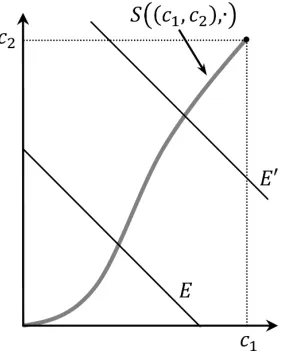
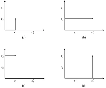
A convenient way of graphically representing a division rule is the path of awards it generates. For a fixed set of claimants N and for a fixed claims vector c for those claimants, the path of awards of a rule S is the graph of all possible allocations awarded by S as E varies from 0 to the sum of claims P
Nci. See Figure 1.
Alternatively, a problem (c, E) can be interpreted as a cost-sharing problem or a taxation problem. Under the cost-sharing interpretation, cis the vector of monetary benefits each individual will receive from the shared project andE is the cost of the project. The restriction E ≤ P
Nci means that the project is socially beneficial.
Under the taxation interpretation, c is the vector of incomes and E is the total tax to be raised.
2.2
Examples of Division Rules
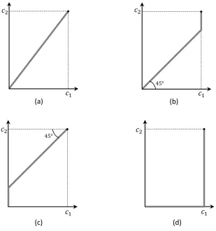
The following are simple examples of division rules. Figure 2 illustrates the paths of awards for each of these division rules.
• The Proportional Rule. For every (c, E) and for every i∈N,
Figure 1: Path of awards. The horizontal axis measures claimant 1’s claim and award. The vertical axis measures claimant 2’s. The path of awards is the set of all
awards as E varies.
whereλis chosen so thatP
NPj(c, E) =E. (Note then thatλ =E P
Ncj.)P
gives to each claimant the same proportion of his respective claim. For example, if there is only enough of the endowment to cover half of the total claims, then
P will give each claimant half of his claim.
• The Constrained Equal Awards Rule. For every (c, E) and for every i∈N,
CEAi(c, E)≡min{ci, λ}
where λ is chosen so that P
NCEAj(c, E) = E. CEA gives to each claimant
the same award, with the exception of those claimants who would otherwise receive more than their respective claims.
• The Constrained Equal Losses Rule. For every (c, E) and for every i∈N,
CELi(c, E)≡max{0, ci−λ},
where λ is chosen so thatP
NCELj(c, E) =E. CEL equalizes losses (i.e. the
difference between an agent’s claim and his award) across claimants, with the exception of those claimants who would otherwise receive a negative award.
• The Dictatorial Rule with priority (where is a strict linear order overN). For every (c, E) and for every i∈N,
Dici (c, E)≡
ci, if iλ
E−P
j∈N:jicj, if i=λ
0, if λi
,
where λ ∈ N is chosen so that P NDic
j (c, E) = E. Dic distributes the
Figure 2: Paths of awards for examples. The paths of awards for (a) P, (b)
CEA, (c) CEL, and (d) Dic12.
3
Main Results
3.1
Asymmetric Parametric Division Rules
We characterize a family of division rules that we call (asymmetric)parametric rules. To understand this family, consider again the examples above. In each case, the award given to a claimant is determined by his claim ci and a parameter λ. For a given
problem, a common parameter is chosen for all claimants so that the sum of awards equals the endowment.
Formally, let F be the family of functions f : N×R++ ×[a, b] → R+, where −∞ ≤ a < b≤ ∞, such that (i) f is weakly increasing in the third argument, (ii)f
is continuous in the third argument, and (iii) for everyi ∈N and c0 ∈R++ we have f(i, c0, a) = 0 and f(i, c0, b) =c0. From here on, we will write f(i, ci, λ) as fi(ci, λ).
One can alternatively think of f ∈ F as the collection of functions{fi}N, where each
fi :R++×[a, b]→R+ satisfies the above three criteria.
Observe that for anyf ∈ F and for any claims vector c, the function P
Nfi(ci,·)
is continuous and weakly increasing. So by the Intermediate Value Theorem, for every (c, E) there exists λ∈[a, b] such thatP
Nfi(ci, λ) =E. Moreover, if λ
0 is such that
P
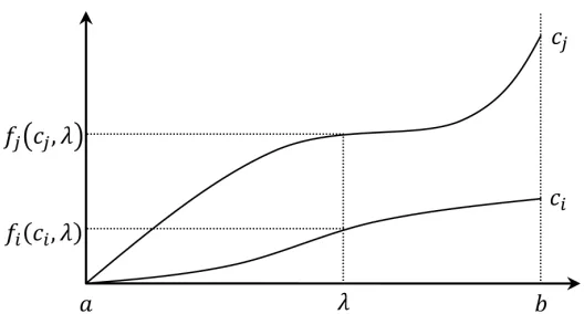
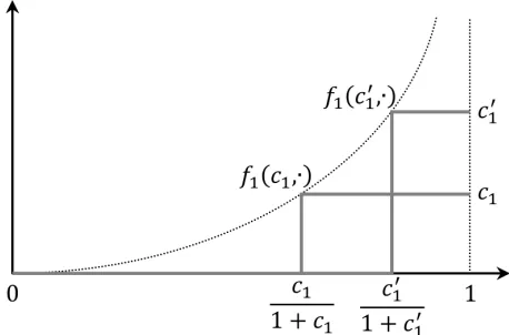
Figure 3: Parametric functions. An asymmetric parametric division rule would divide E between i and j (when their respective claims are ci and cj) by finding λ
such that fi(ci, λ) +fj(cj, λ) =E.
for any f ∈ F, we can define a division rule Sf as follows. For every (c, E) and for
every i∈N,
Sif(c, E)≡fi(ci, λ) , (1)
where λ is chosen so that P
Nfi(ci, λ) = E. We say a rule S has a parametric
representation if there existsf ∈ F such that S=Sf. If f is continuous then we say
S has a continuous parametric representation. See Figure 3.
A special case is a rule that has a parametric representation f ={f0}, i.e. where fi = f0 for every i ∈ N. We say S has a symmetric parametric representation f0
if {f0} ∈ F is a parametric representation of S. Such rules were characterized by
Young (1987), and we discuss his axioms shortly.
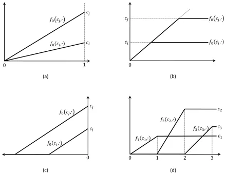
Of our examples above, P, CEA, and CEL all have symmetric parametric rep-resentations, while Dic has an asymmetric parametric representation. For P, the function
f0(ci, λ) = λci
is a parametric representation where a= 0 andb = 1. ForCEA, the function
f0(ci, λ) = min{ci, λ}
is a parametric representation where a= 0 andb =∞. For CEL, the function
f0(ci, λ) = max{0, ci+λ}
is a parametric representation where a = −∞ and b = 0. For Dic< (note that is
the “less than” relation), the collection of functions
fi(ci, λ) =
0, λ < i−1 (1 +λ−i)ci, i−1≤λ < i
ci, λ≥i
Figure 4: Parametric representations for examples. Parametric representa-tions of (a) P, (b) CEA, (c) CEL, and (d) Dic<.
3.2
Young (1987)
As parametric rules are a generalization of Young’s (1987) symmetric parametric rules, we first introduce the axioms used by Young. One of the most prominent axioms studied in the literature is Consistency, which deals with how the rule allocates when the group of claimants shrinks.
Consistency. For every (c, E), if N0 ⊂N, then
SN0(c, E) =S(cN0,P
N0Si(c, E)).
A slightly weaker version is Bilateral Consistency, which is Consistency applied only to two-person subgroupsN0.
To understand Consistency, consider the following. Suppose a rule chooses an allocation for a problem. Some claimants are given their respective awards and leave. Suppose now the rule is asked to reconsider its original allocation for those claimants who remain. That is, the rule is given the opportunity to reallocate what remains of the endowment between the claimants who have not yet received their awards.4 The
4This is also a claims problem sinceP
N0Si(c, E)≤
P
rule can choose to distribute according to the original allocation, or it can choose a new allocation. What Consistency says is that the rule will always choose the original allocation. All of the examples given above are consistent, though it would not be difficult to construct a rule that is not. For example, a rule that distributed according toCEAwhen there are three claimants andCELwhen there are two claimants would not satisfy Consistency.
Symmetry. For every (c, E) and for every {i, j} ⊂ N, if ci = cj, then Si(c, E) =
Sj(c, E).
This states that if two agents have the same claim, then they will get the same award. Of the examples above, Dic is not symmetric.
Continuity. For every (c, E), for every sequence of problems ck, Ek with the same group of claimants N, if ck, Ek
→(c, E), then S ck, Ek
→S(c, E).
Young’s Theorem states that a division rule has a continuous symmetric para-metric representation if and only if it satisfies Continuity, Bilateral Consistency, and Symmetry. An important step in the proof is showing that these three axioms imply the following.
Resource Monotonicity. For every (c, E) and (c, E0), if E < E0, then for every
i∈N we have Si(c, E)≤Si(c, E0).
Resource Monotonicity states that if the endowment increases, no claimant should get a smaller award. A stronger version is Strict Resource Monotonicity, the only difference being a strict rather than weak inequality in the statement of the axiom. All of the examples given above are resource monotonic, while P is also strictly resource monotonic.
3.3
Intrapersonal Consistency
We motivate our first novel axiom with the following example, which illustrates that simply dropping Symmetry from Young’s theorem is not enough to characterize para-metric rules.
Example 1 We construct a continuous, consistent, and resource monotonic rule and show that it does not have a parametric representation.
Consider the rule S defined over any claims problem where N = {1,2}. Fix c1, c01, c2, and c02 where c1 < c01 and c2 < c02. Let S satisfy S((c1, c2), c1) = (c1,0), S((c01, c2), c2) = (0, c2), S((c1, c02), c
0
2) = (0, c
0
2), and S((c
0
1, c
0
2), c
0
1) = (c
0
1,0). Hence,
if claims are either(c1, c2)or(c01, c
0
2)thenS gives priority to claimant1over claimant
2. If claims are either (c01, c2) or (c1, c02) then S gives priority to 2 over 1. Figure 5
illustrates the paths of awards for this rule.
In the appendix, we show that S can be extended to a continuous, consistent, and resource monotonic rule over all problems.
Figure 5: Paths of awards for Example 1. Panel (a) shows that when 1 has claim c1 and 2 has claim c2, then 1 is given priority over 2. Panel (b) shows that
when1 has a claim ofc01 and 2has a claim ofc2, then2 is given priority over 1. Etc.
increasing on [λ, λ0], f1(c1, λ) = 0, f1(c1, λ0) = c1, and where f2(c2,·) is zero on
[λ, λ0]. Similarly, panel (b) would imply that there exists λ00 > λ0 such that f2(c2,·)
is weakly increasing on [λ0, λ00], f2(c2, λ00) = c2, and where f1(c01,·) is zero on [λ, λ
00]. Panel (d) would imply that there existsλ000 > λ00 such thatf1(c01,·)is weakly increasing
on [λ00, λ000], f1(c01, λ
000) =c0
1, and where f2(c02,·) is zero on [λ, λ
000]. Finally, panel (c) would imply that f1(c1,·) is zero on[λ, λ000], which is a contradiction since we already
showed that f1(c1, λ0) =c1.
The key to understanding this example is recognizing that a rule can implicitly reveal how it allocates between different claims of one claimant. For example, panel (a) of Figure 5 shows thatS gives priority to c1 overc2, while panel (b) shows thatS
gives priority to c2 overc01. Hence, S implicitly gives priority to c1 overc01. However, S fails to have an asymmetric parametric representation because panels (c) and (d) imply the opposite: that S gives priority to c01 over c1. The reason why Consistency
does not preclude such rules is because it has no force with two-person groups. What is needed is an axiom that requires a rule to be intrapersonally consistent.
The following definitions will make it easier to formalize this axiom. Define:
Figure 6: Illustration of G.
We think of (i, ci, xi) as describing an agent, his claim, and his award. Following
Young (1994, p.76), we will call (i, ci, xi) a situation.5 For a given rule S, for every
situation (i, ci, xi)∈Y, j 6=i, and cj ∈R++, define the function: G((i, ci, xi), j, cj)≡inf{E :Si((ci, cj), E)≥xi}.
Figure 6 illustrates.
Observe that for continuous rules, inf can be replaced with min. HenceG((i, ci, xi), j, cj)
is the smallest endowment needed for S to award xi to agent i (when i’s and j’s
re-spective claims are ci and cj).
Define the binary relation R1 overY as follows.
Definition 1 (i, ci, xi)R1(j, cj, xj)ifi6=j andG((i, ci, xi), j, cj)≤G((j, cj, xj), i, ci).
Let I1 and P1 denote the symmetric and asymmetric parts of R1 respectively.
Obviously, (i, ci, xi)I1(j, cj, xj) if and only if G((i, ci, xi), j, cj) = G((j, cj, xj), i, ci)
and (i, ci, xi)P1(j, cj, xj) if and only if G((i, ci, xi), j, cj)< G((j, cj, xj), i, ci).
Consider Figure 6 again. As the endowment increases from 0 toc1+c2, the amount
awarded follows the path of awards from the origin to (c1, c2). The path crosses the
vertical line representingx1 before it crosses the horizontal line representingx2.
(Ob-serve that this particular division rule is not resource monotonic, and so the path of awards crossesx1multiple times.) This means the rule awardsx1 to 1 before it awards x2 to 2, or (1, c1, x1)P1(2, c2, x2). In this sense, we think of R1 as being (part of) an
underlying social preference over situations that determines how a rule adjudicates problems. That is, if (i, ci, xi)R1(j, cj, xj), then presumably this is because the rule
deems it just to award xi toi before it awardsxj to j (when their respective claims
are ci and cj).
5Note however that since Young assumes Symmetry, his definition of a situation does not include
the individual’s identity. That is he defines a situation as the pair (c0, x0) where c0 > 0 and
However R1 is not a complete ordering as it requires thati6=j. That is, R1 does
not make intrapersonal comparisons directly. But as illustrated in Example 1, a rule’s social preference over intrapersonal situations can be revealed indirectly. That is, if we have (i, ci, xi)P1(j, cj, xj) and (j, cj, xj)P1(i, c0i, x
0
i), then we can interpret that as
saying there is a social preference of (i, ci, xi) over (i, c0i, x
0
i) even though there is no
claims problem that would reveal that social preference directly. This brings us to our axiom.
Intrapersonal Consistency. For every(i, ci, xi),(i, c0i, x
0
i),(j, cj, xj), j, c0j, x
0
j
∈Y
where i6=j, if
(i, ci, xi)P1(j, cj, xj)P1(i, c0i, x
0
i),
then it is not true that
(i, c0i, x0i)P1 j, c0j, x
0
j
P1(i, ci, xi).
Intrapersonal Consistency is a restriction on how the rule implicitly allocates be-tween different claims of the same claimant. It states that if there is a social preference for (i, ci, xi) over (i, c0i, x
0
i), then there cannot also be a social preference for the
oppo-site.6 Obviously Example 1 violates Intrapersonal Consistency.
To understand how Intrapersonal Consistency relates to Consistency, consider the following variation.
Alternative to Consistency. For every (i, ci, xi),(j, cj, xj),(k, ck, xk),(l, cl, xl) ∈
Y where i, j, k are distinct and i, k, l are distinct, if
(i, ci, xi)P1(j, cj, xj)P1(k, ck, xk),
then it is not true that
(k, ck, xk)P1(l, cl, xl)P1(i, ci, xi).
This alternative to Consistency concerns interpersonal comparisons, as opposed to the intrapersonal comparisons in Intrapersonal Consistency. One can show that Consistency implies the above alternative.7 Conversely, one could replace Consistency with the above alternative in Theorem 1 and the result would still hold.
We now formalize the implicit intrapersonal ranking of a rule. Define the binary relationR2 overY as follows.
6Though stated as a restriction on the ordering R
1, Intrapersonal Consistency is a
restric-tion on division rules since R1 is defined from S. The statement of the axiom purely in terms
of (continuous) division rules is as follows: For every {i, j} ⊂ N, ci, c0i, cj, c0j ∈ R++, and
E, E0,E,ˆ Eˆ0 ∈R+, ifS((ci, cj), E) = (xi, xj), S((c0i, cj), E0) = x0i, x0j
,S ci, c0j,Eˆ= (xi,xjˆ ),
S c0i, c0j
,Eˆ0= x0i,xˆ0j
,E=G((i, ci, xi), j, cj),E0=G((i, ci, x0i), j, cj), ˆE=G (i, ci, xi), j, c0j
,
ˆ
E0=G (i, c
i, x0i), j, c0j
, andxj < x0j, then ˆxj ≤xˆ0j.
Figure 7: “Parametric” representation for Example 2. f1 is a collection of
step correspondences.
Definition 2 (i, ci, xi)R2(i, c0i, x0i)if there exists (j, cj, xj)∈Y where j 6=isuch that
(i, ci, xi)R1(j, cj, xj)R1(i, c0i, x
0
i).
Let I2 and P2 denote the symmetric and asymmetric parts of R2 respectively.
Define the binary relation C overY as follows.
Definition 3 (i, ci, xi)C(i, c0i, x
0
i)if either(i, ci, xi)R2(i, c0i, x
0
i)or(i, c
0
i, x
0
i)R2(i, ci, xi).
So we interpretCto be the “comparable” relation. That is, situations (i, ci, xi) and
(i, c0i, x0i) are comparable if there exists some (j, cj, xj) that separates them. However
it may be that such a (j, cj, xj) does not exist, in which case (i, ci, xi) and (i, c0i, x
0
i)
would not be comparable. Let N C denote the “not comparable” relation.
3.4
Non-comparability Continuity in Claims at Priority Points
Our final axiom concerns when two situations should not be comparable. To motivate this axiom, consider the following example.
Example 2 We construct a rule that is continuous, consistent, intrapersonally con-sistent, and resource monotonic, but which does not have a parametric representation. For i6= 1, let fi(c0, λ) = λc0 be i’s parametric function on [0,1]. For i= 1, f1 is not
a function, but rather a correspondence on [0,1], defined by
f1(c0, λ) =
0, for λ < c0 1+c0
[0, c0] for λ= 1+c0c0 c0, for λ > 1+c0c0
.
So for every c0, f1(c0,·) is a step correspondence where 1+c0c0 is the location of the
step and c0 is its height. Figure 7 illustrates f1.
Observe that for any (c, E), there exists a unique λ such that E ∈P
i∈N fi(ci, λ).
So define a division rule S as follows. For any (c, E), for i6= 1,
and for i= 1,
S1(c, E)≡E−
X
i∈N\{1}
Si,
where λ is chosen so that E ∈ P
i∈Nfi(ci, λ). (Hence, S1(c, E) ∈ f1(c1, λ).) One
can show that S is continuous, consistent, intrapersonally consistent, and resource
monotonic.
We claim that S does not have an asymmetric parametric representation. Suppose
it does have a representation, fˆ. For every c0 >0, set m(c0)≡sup
n
λ∈[a, b] : ˆf1(c0, λ) = 0
o
and
M(c0)≡inf
n
λ∈[a, b] : ˆf1(c0, λ) = c0
o
.
Hence, [m(c0), M(c0)] is the smallest subinterval of [a, b] such that the range of
ˆ
f1(c0,·) is [0, c0]. Since fˆ1 is continuous in the second argument, m(c0) < M(c0)
for every c0 > 0. By definition of S, if c0 < c00, then M(c0) < m(c00). (This is
because for claimant 1, S gives priority to smaller claims.) Let Q denote the set of rational numbers. Since Q is dense inR, choose q(c0)∈[m(c0), M(c0)]∩Q for every c0. By above, if c0 < c00, then q(c0)< q(c00). Hence{q(c0) :c0 >0} is an uncountable
set of distinct rational numbers, which is impossible since Q is countable.
Before stating the axiom, we need a definition.
Definition 4 The rule S gives priority to (i, ci, xi) ∈Y if xi ∈ (0, ci) and if
there exists > 0 such that for every (ˆc, E) where i ∈N, cˆi =ci, and Si(ˆc, E) = xi,
for every a ∈(−, ),
Si(ˆc, E +a) =xi+a.
Though this definition may seem very restrictive, there are many rules which give priority to some situation. For example, Dic gives priority to every (i, ci, xi) where
xi ∈ (0, ci). Similarly, in Example 2, the rule gives priority to every (1, c1, x1) where x1 ∈(0, c1).
Non-comparability Continuity in Claims at Priority Points. If S gives pri-ority to (i, ci, xi), then there exists > 0 such that for every c0i ∈ (ci−, ci+), we
have (i, c0i, xi)N C(i, ci, xi).
We will refer to this axiom as N-Continuity. If S gives priority to situation (i, ci, xi), then small perturbations of xi will not be comparable to (i, ci, xi).
N-Continuity states that if such is the case, then small perturbations of ci will also not
be comparable to (i, ci, xi). Though certainly not intuitive, this technical axiom is
3.5
Characterizations and Independence of Axioms
We now state the main theorem.
Theorem 1 S has a continuous parametric representation if and only if S satis-fies Continuity, N-Continuity, Bilateral Consistency, Intrapersonal Consistency, and Resource Monotonicity.
The basic outline of the proof is not hard to understand. Using R1 and R2, we
define a complete ordering R over Y. Consistency and Intrapersonal Consistency imply that R is also transitive. Continuity and N-Continuity imply that there is a countableR-dense subset of Y. Thus, by the standard representation result, there is a numerical representation r :Y →R of R. The function r thus acts as a numerical measure of the fairness of a situation, just as the parameter in the parametric function acts as a measure of fairness. Thus taking the inverse of r with respect to the third argument (the award) gives us the parametric function. The remainder of the proof is to show that this does in fact represent the division rule and that it satisfies the properties of a parametric function.8
The following examples demonstrate the extent to which the axioms are indepen-dent. (Verification that each example satisfies all the axioms but the one stated is left to the reader.)
• Continuity. A division rule that satisfies all the axioms but Continuity is as follows. Let f ∈ F be such that fi is strictly increasing in λ but not jointly
continuous for every i. Define S according to (1). Then S is not continuous. However, since fi is strictly increasing inλ for everyi, there is no (i, ci, xi)∈Y
such that S gives priority to (i, ci, xi). So N-Continuity is satisfied vacuously.
The other axioms can be easily verified.
• N-Continuity. Example 2 satisfies all the axioms but N-Continuity.
• Bilateral Consistency. A division rule which allocates according to P for two-person groups, but CEA for groups larger than two, would satisfy all the axioms but Consistency.
• Intrapersonal Consistency. Example 1 satisfies all the axioms but Intraper-sonal Consistency.
It is an open question whether Resource Monotonicity is independent of the other axioms.
8Other papers use similar techniques of using an ordering over an appropriately defined situation
If Resource Monotonicity is strengthened to Strict Resource Monotonicity, then the parametric representation is strictly increasing in the parameter. However, it is interesting to note that for strictly resource monotonic rules, the axioms Intrapersonal Consistency and N-Continuity are not needed for the characterization.
Theorem 2 S has a continuous parametric representation with a strictly increasing parametric function if and only if S satisfies Continuity, Bilateral Consistency, and Strict Resource Monotonicity.
3.6
Parametric Rules and Collective Rationality
Choosing an award that maximizes some measure of social welfare is a natural way of solving a claims problem. In this section, we show that every parametric division rule maximizes a continuous, strictly convex, additively separable social welfare function. Young (1987, Theorem 2) has a similar result, though obviously without symmetry.
In our setting, a social welfare function (SWF) is a real-valued function W of claims-awards pairs (c, x). We say a SWF is additively separable if there exists U :
Y →R such thatW(c, x) = P
i∈N Ui(ci, xi). Note that if U is strictly concave in the
third argument, then for every claims problem (c, E), arg maxx∈X(c,E)
P
i∈NUi(ci, xi)
is a singleton.9 Hence for such a U, we can define a division rule:
SU(c, E)≡arg max
x∈X(c,E)
X
i∈N
Ui(ci, xi).
We say a division rule S has a collectively rational additively separable (CRAS) rep-resentation if there existsU :Y →Rstrictly convex in the third argument such that
S =SU. If U is continuous, then we sayS has a continuous CRAS representation.
Theorem 3 S has a continuous parametric representation if and only if S has a continuous CRAS representation.
Together, Theorems 1 and 3 imply that Continuity, N-Continuity, Bilateral Consis-tency, Intrapersonal ConsisConsis-tency, and Resource Monotonicity characterize the family of continuous CRAS rules.
The intuition behind the proof can provide insight into the connection between these two families of rules. Begin with a CRAS rule. The first order conditions for the maximization problem require that the solution equalize marginal utilities between all claimants who are not constrained by their respective claims. Taking the inverse of each claimants marginal utility function with respect to their award gives us their parametric function. Going the other direction, if a rule has a parametric representation, then taking the inverse of each claimants parametric function with respect to the parameter gives us what will become their marginal utility function. Integrating that gives us each claimant’s utility function, which we add together to get the additively separable SWF.
9Recall thatX(c, E) ={x:P
The key insight here is that the marginal utility function plays the same role as the ordering R that we construct for the proof of Theorem 1. Specifically, if (i, ci, xi)
gives a higher marginal utility than (j, cj, xj), then in order to maximize social welfare,
a CRAS rule must allocate xi to i before it allocates xj to j when their respective
claims are ci and cj. But this is exactly what (i, ci, xi)R(j, cj, xj) means. Hence the
marginal utility function and r, the numerical representation of R, are essentially interchangeable, and this fact is exploited in the proof for Theorem 3.
This also provides us with a new interpretation of a parametric rule. Namely a parametric rule divides by assigning to each claimant a utility function, and then finds an award so as to equalize marginal utilities across the claimants subject to the constraint that no claimant receive more than his claim. In this interpretation, the parameter – the measure of fairness by which the division rule compares situations – is the marginal utility that each claimant receives at his award. Thus the rule treats the claimants fairly be equalizing their marginal utilities.
This method of solving a claims problem is similar to the one characterized by Lensberg (1987) for bargaining problems. Indeed, one could view the family of claims problems as a special class of bargaining problems. One key difference is that here the SWF depends on the individual’s claims, something which is not present in Lensberg’s result.
We finish with a result for strictly resource monotonic division rules.
Theorem 4 S has a continuous parametric representation with a strictly increasing
parametric function if and only if S has a continuous CRAS representation that is
continuously differentiable in the third argument.
Together, Theorems 2 and 4 imply that Continuity, Bilateral Consistency, and Strict Resource Monotonicity characterize this family of division rules.
4
Concluding Remarks
We conclude by discussing an alternative characterization of the parametric family of division rules. This alternative characterization requires an expanded definition of a claims problem, but standard (appropriately modified) axioms. To do this, we employ a result due to Kaminski (2006).
As discussed in the introduction, the definition of a problem does not allow a di-vision rule to make direct intrapersonal allocations. We have followed this traditional formulation of a problem, and our two novel axioms, Intrapersonal Consistency and N-Continuity, impose restrictions on how a rule indirectly allocates intrapersonally. An alternative approach would be to expand the definition of a problem to directly al-low for such intrapersonal allocations, and then impose standard axioms. We outline how that might be formulated.
For a finite group of claimants N ⊂ N, a problem is a tuple (m, c, E) where
m ∈ NN is the vector of identities of the claimants, c ∈
RN++ is the vector of their
avoid confusion with the traditional formulation of a claims problem, we call (m, c, E) anexpanded claims problems.
The main difference here is in how a claimant’s identity is encoded in a problem. Earlier,i∈N represented the identity of a claimant. Now,i∈N simply enumerates a claimant (we refer toias the claimant’s “number”), whilemi represents the identity
of the ith claimant. Hence, ifm1 =m2, then we interpret this to mean that claimant
number 1 and claimant number 2 are the same individual. Thus a division rule can make direct intrapersonal allocations.
An expanded claims problem is actually a special case of the problems formulated by Kaminski (2006) (though this special case was not one originally considered by Kaminski). In that paper, there is a type space T, which has no structure other than being a separable topological space. Each individual i has a type ti ∈ T. There is
also a function max : T → R++∪ {∞} which determines the maximum award each
type may receive, i.e. an award xi ≥ 0 for individual i is valid if xi ≤ max(ti). For
a group N ⊂N, a problem is the tuple (t, E)∈TN ×R++, where E ≤
P
Nmax(ti).
This generalization allows for many different applications.10 For our purposes, an individual’s type will be his identitymi and claimci, and the maximum an individual
can receive will be his claim. Thus we have T =N×R++ and max(mi, ci) =ci.
As before, for any f ∈ F, we can define a division rule Sf as follows. For every (m, c, E) and for every i∈N,
Sif(m, c, E)≡fmi(ci, λ), (2)
whereλis chosen so thatP
i∈Nfmi(ci, λ) =E. Note that here, though the parametric
functionf belongs to the same family of functions F as before, the first input off is now mi rather than i.
We impose the same axioms as Young (1987), appropriately modified. Continuity and Bilateral Consistency are essentially the same as before. However Symmetry takes on a different meaning here.
Symmetry. For every (m, c, E) and {i, j} ⊂ N, if mi = mj and ci = cj, then
Si(m, c, E) = Sj(m, c, E).
Here, Symmetry is considerably weaker than earlier because claimants with the same claim but different identities can receive different awards. It is only to “clones” (i.e. claimants with the same identity and claim) that the division rule must give the same award. However, Symmetry still imposes quite a bit of richness on the rule since it implies, with Continuity and Bilateral Consistency, appropriate adaptations of both N-Continuity and Intrapersonal Consistency.
Applying Kaminski (2006, Theorem 1), we get an alternative characterization of our family of parametric rules: A division rule over expanded claims problems satisfies
10Some applications that Kaminski cites: (1) Claims problems: T =
R++ and max(t0) =t0. (2)
Surplus sharing: T = R++ and max(t0) = ∞. (3) Multiple claims: T = RK++ where K is the
number of different claim types and max(t0) =P
K k=1t
k
0. (4) Welfarist rationing: T is the set of all
Continuity, Bilateral Consistency, and Symmetry if and only if it has a continuous parametric representation of the form given in (2).11
Though this approach to characterizing parametric rules has the advantage of using simpler, well-known axioms, it has the disadvantage of being arguably unrealis-tic. What does it mean to have multiple versions of the same claimant in a problem? Also it obscures the intrapersonal properties that parametric rules satisfy under the traditional formulation of a claims problem.
11To see that this is a characterization of the same family of rules, first observe that the set
Appendix
A
Continuing Example 1
Here we show thatS, the division rule in Example 1, can be extended to a continuous, consistent, and resource monotonic rule over all problems. First we show that there is a continuous extension of S for problems where N ={1,2}. Later we will extend
S to the domain of all problems.
For now, S is only defined over problems where N = {1,2}. Here we show that there is a continuous extension of S given S((c1, c2), c1) = (c1,0), S((c01, c2), c2) =
(0, c2),S((c1, c02), c02) = (0, c02), andS((c01, c02), c01) = (c01,0). We do this by describing
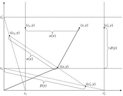
the path of awards for any problem. Every path of awards will be piecewise linear of exactly two pieces: the first piece starting at the origin, the second piece ending at the claims vector, and the two meeting somewhere in between at an inflection point. Thus for any claims vector (x, y), the path of awards will be defined by the inflection point i(x, y) lying somewhere in the box formed by the origin and (x, y). This guarantees that the rule is resource monotonic. Also, the inflection point will vary continuously with respect to claims, guaranteeing the rule is continuous.
In what follows, set:
α(x)≡
0 if x≤c1 x−c1
c01−c1
if c1 < x≤c01
1 if x > c01
and
β(y)≡
0 if x≤c2 y−c2
c02−c2
if c2 < x≤c02
1 if x > c02. Now set:
i(x, y)≡((1−α(x))(1−β(y)) min{x, c1}+α(x)β(y) max{x, c01}, α(x)(1−β(y)) min{y, c2}+ (1−α(x))β(y) max{y, c02}) .
Observe that i(c1, c2) = (c1,0), which is what is required given thatS((c1, c2), c1) =
(c1,0). Similarly we have i(c01, c2) = (0, c2), i(c1, c02) = (0, c
0
2), and i(c
0
1, c
0
2) = (c
0
1,0).
Also, observe that for x∈ (c1, c01) and y ∈(c2, c02), we can write i(x, y) in one of two
ways: either as the α(x) mixture of i(c1, y) and i(c01, y), or as the β(y) mixture of i(x, c2) and i(x, c02). Figure 8 illustrates.
It is straightforward to show that 0≤i1(x, y)≤xfor everyx >0, 0≤i2(x, y)≤y
for every y > 0, and that i(x, y) is continuous. Thus S is continuous and resource monotonic.
( ) ( )
( )
( )
( ) ( )
( ) ( )
( )
[image:22.612.112.508.79.389.2]( )
Figure 8: Construction of path of awards. The path of awards for claims vector
(x, y) is shown. Note that i(x, y) is the convex combination of i(c1, y) and i(c01, y).
rule). For any other problem (where 1 ∈ N, 2 ∈ N, or 1,2 ∈ N), S divides the endowment by first satisfying the claims of claimants 1 and 2, dividing between them as above if 1,2 ∈ N, and then allocating the remainder of the endowment to the rest of the claimants according to P ar. It is not hard to show that S is continuous, consistent, and resource monotonic. However as shown previously, S cannot have a parametric representation.
B
Proof of Theorem 1
B.1
Preliminaries
Set
m(i, ci, xi)≡inf{x0i ≤xi : (i, ci, x0i)N C(i, ci, xi)}
and
M(i, ci, xi)≡sup{x0i ≥xi : (i, ci, x0i)N C(i, ci, xi)}
and
θ(i, ci, xi)≡ (
0 if m(i, ci, xi) =M(i, ci, xi) xi−m(i,ci,xi)
M(i,ci,xi)−m(i,ci,xi) if m(i, ci, xi)< M(i, ci, xi)
.
When they are well-defined, m(i, ci, xi)≤xi ≤M(i, ci, xi) and 0≤θ(i, ci, xi)≤1.
Lemma 1 If (i, ci, xi)N C(i, c0i, x0i), then m(i, ci, xi), M(i, ci, xi), and θ(i, ci, xi)are
well-defined.
Proof. If (i, ci, xi)N C(i, c0i, x0i), then there exists no (j, cj, xj) such that (i, ci, xi)I1(j, cj, xj).
Hence (i, ci, xi)N C(i, ci, xi), which implies
xi ∈ {x0i ≤xi : (i, ci, x0i)N C(i, ci, xi)}
and
xi ∈ {x0i ≥xi : (i, ci, x0i)N C(i, ci, xi)}.
Define the binary relation R3 overY as follows.
(i, ci, xi)R3(i, c0i, x
0
i) if (i, ci, xi)N C(i, c0i, x
0
i) and θ(i, ci, xi)≤θ(i, c0i, x
0
i) .
DefineR ≡R1∪R2∪R3. Lemma 2 R is complete.
Proof. For every (i, ci, xi) and (j, cj, xj), either (i) i 6= j, (ii) i = j and (i, ci, xi)C
(j, cj, xj), or (iii)i=jand (i, ci, xi)N C(j, cj, xj). If (i), then eitherG((i, ci, xi), j, cj)≤
G((j, cj, xj), i, ci) or G((i, ci, xi), j, cj) ≥ G((j, cj, xj), i, ci). If (ii), then (i, ci, xi)C
(j, cj, xj) implies either (i, ci, xi)R2(j, cj, xj) or (j, cj, xj)R2(i, ci, xi). If (iii), then
either θ(i, ci, xi)≤θ(j, cj, xj) or θ(i, ci, xi)≥θ(j, cj, xj).
B.2
R
Is Transitive
Lemma 3 For every (i, ci, xi)∈Y, j 6=i, and cj ∈R++, we have Si((ci, cj), G((i, ci, xi), j, cj)) =xi.
Lemma 4 For every i, j, k distinct, for every ci, cj, ck ∈ R++, for every xi ∈ [0, ci],
there exists E such that
S((ci, cj, ck), E) = (xi, G((i, ci, xi), j, cj)−xi, G((i, ci, xi), k, ck)−xi).
Proof. Set
E ≡G((i, ci, xi), j, cj) +G((i, ci, xi), k, ck)−xi
and
x0i, x0j, x0k
≡S((ci, cj, ck), E) .
Hence,
x0i+x0j +x0k=G((i, ci, xi), j, cj) +G((i, ci, xi), k, ck)−xi. (3)
First we show x0i = xi. Suppose x0i < xi. Observe that Bilateral Consistency
implies S (ci, cj), x0i+x
0
j
= x0i, x0j and S((ci, ck), x0i+x
0
k) = (x
0
i, x
0
k). Also, by
Lemma 3,
S((ci, cj), G((i, ci, xi), j, cj)) = (xi, G((i, ci, xi), j, cj)−xi)
and
S((ci, ck), G((i, ci, xi), k, ck)) = (xi, G((i, ci, xi), k, ck)−xi) .
Since x0i < xi, Resource Monotonicity implies x0j ≤G((i, ci, xi), j, cj)−xi and x0k ≤
G((i, ci, xi), k, ck)−xi. Hence,
x0i+x0j +x0k< G((i, ci, xi), j, cj) +G((i, ci, xi), k, ck)−xi,
which contradicts equation (3). The proof is similar if x0i > xi. Hence x0i =xi.
Now we show x0j = G((i, ci, xi), j, cj)−xi and x0k = G((i, ci, xi), k, ck)−xi. By
definition ofG,xi+x0j ≥G((i, ci, xi), j, cj) andxi+x0k ≥G((i, ci, xi), k, ck). If either
of these inequalities are strict, then
xi+x0j +x
0
k> G((i, ci, xi), j, cj) +G((i, ci, xi), k, ck)−xi,
which contradicts equation (3). Hence, xi +x0j = G((i, ci, xi), j, cj) and xi +x0k =
G((i, ci, xi), k, ck).
Lemma 5 (i, ci, xi)P1(j, cj, xj) if and only if xi+xj > G((i, ci, xi), j, cj).
Proof. By Lemma 3,
S((ci, cj), G((i, ci, xi), j, cj)) = (xi, G((i, ci, xi), j, cj)−xi)
and
S((ci, cj), G((j, cj, xj), i, ci)) = (G((j, cj, xj), i, ci)−xj, xj) .
(⇒) So G((i, ci, xi), j, cj) < G((j, cj, xj), i, ci). Resource Monotonicity implies
G((i, ci, xi), j, cj)−xi ≤xj. If G((i, ci, xi), j, cj)−xi =xj, then
But this would imply G((i, ci, xi), j, cj) ≥ G((j, cj, xj), i, ci) by definition of G, a
contradiction. Hence, G((i, ci, xi), j, cj)−xi < xj.
(⇐) Suppose xj > G((i, ci, xi), j, cj)−xi. Then Resource Monotonicity implies
G((i, ci, xi), j, cj)<((j, cj, xj), i, ci), or (i, ci, xi)P1(j, cj, xj).
Observe that an alternative statement of Lemma 5 is (i, ci, xi)R1(j, cj, xj) if and
only if xi+xj ≤G((j, cj, xj), i, ci).
Lemma 6 If (i, ci, xi)N C(i, ci, x0i), thenm(i, ci, xi) =m(i, ci, xi0)andM(i, ci, xi) =
M(i, ci, x0i).
Proof. Follows immediately from transitivity of N C.
Lemma 7 (i, ci, xi)R(i, ci, x0i) if and only if xi ≤x0i.
Proof. Case 1: (i, ci, xi)C i, ci, x0i
. So there exists (j, cj, xj) such that
(i, ci, xi)R1(j, cj, xj)R1(i, ci, x0i) .
This is true if and only ifG((i, ci, xi), j, cj)≤G((j, cj, xj), i, ci)≤G((i, ci, x0i), j, cj).
But Resource Monotonicity impliesG((i, ci, xi), j, cj)≤G((i, ci, x0i), j, cj) if and only
if xi ≤x0i.
Case 2: (i, ci, xi)N C i, ci, x0i
.
By Lemma 6,m(i, ci, xi) = m(i, ci, x0i) andM(i, ci, xi) = M(i, ci, xi0). Ifm(i, ci, xi) =
M(i, ci, xi), then 0 = θ(i, ci, xi) = θ(i, ci, x0i) andm(i, ci, xi) = M(i, ci, xi) =xi =x0i.
Ifm(i, ci, xi)< M(i, ci, xi), then the definition of θ implies θ(i, ci, xi)≤θ(i, ci, x0i) if
and only if xi ≤x0i.
Lemma 8 If i 6= j and (i, ci, xi)P1(j, cj, xj), then there exists > 0 such that for
every x0j ∈(xj−, xj),
(i, ci, xi)P1 j, cj, x0j
P (j, cj, xj).
Proof. By Lemma 5, (i, ci, xi)P1(j, cj, xj) implies xi+xj > G((i, ci, xi), j, cj). Set
≡xi+xj−G((i, ci, xi), j, cj) .
Then for x0j ∈ (xj −, xj), xi+x0j > G((i, ci, xi), j, cj). So (i, ci, xi)P1 j, cj, x0j
by Lemma 5, while j, cj, x0j
P (j, cj, xj) by Lemma 7.
Lemma 9 If i6=j and (i, ci, xi)P (i, ci, x0i)R1(j, cj, xj), then (i, ci, xi)P1(j, cj, xj).
Proof. Suppose (j, cj, xj)R1(i, ci, xi). Then by definition, (i, ci, x0i)R2(i, ci, xi).
Lemma 7 implies x0i ≤ xi. But (i, ci, xi)P (i, ci, x0i) and Lemma 7 imply xi < x0i,
a contradiction.
Proof. Suppose (i, ci, xi)R(j, cj, xj)R(k, ck, xk).
Case 1: i, j, k distinct.
By Lemma 4, there exists E, E0, and E00 such that
S((ci, cj, ck), E) = (xi, G((i, ci, xi), j, cj)−xi, G((i, ci, xi), k, ck)−xi) ,
S((ci, cj, ck), E0) = (G((j, cj, xj), i, ci)−xj, xj, G((j, cj, xj), k, ck)−xj) ,
S((ci, cj, ck), E00) = (G((k, ck, xk), i, ci)−xk, G((k, ck, xk), j, cj)−xk, xk) .
First we show E ≤E0. If E > E0, then Resource Monotonicity implies
xi ≥G((j, cj, xj), i, ci)−xj,
xj ≤G((i, ci, xi), j, cj)−xi,
and
G((j, cj, xj), k, ck)−xj ≤G((i, ci, xi), k, ck)−xi,
with one of these strict. But G((i, ci, xi), j, cj) ≤ G((j, cj, xj), i, ci). Hence xi =
G((j, cj, xj), i, ci)−xj and xj =G((i, ci, xi), j, cj)−xi, which implies
G((j, cj, xj), k, ck)−xj < G((i, ci, xi), k, ck)−xi (4)
and
S((ci, cj, ck), E0) = (xi, xj, G((j, cj, xj), k, ck)−xj) .
Bilateral Consistency implies
S((ci, ck), xi+G((j, cj, xj), k, ck)−xj) = (xi, G((j, cj, xj), k, ck)−xj) .
By definition,
G((i, ci, xi), k, ck)≤xi+G((j, cj, xj), k, ck)−xj.
But this contradicts inequality (4).
Similarly, E0 ≤ E00. Hence, E ≤ E00. Resource Monotonicity implies xi ≤
G((k, ck, xk), i, ci)−xk andG((i, ci, xi), k, ck)−xi ≤xk. HenceG((i, ci, xi), k, ck)≤
G((k, ck, xk), i, ci), and so (i, ci, xi)R1(k, ck, xk) by definition.
Case 2: i = k6= j.
Then (i, ci, xi)R2(k, ck, xk) by definition.
Case 3: i = j 6=k. So let (i, ci, xi)R(i, c0i, x
0
i)R1(k, ck, xk).
3.1: (i, ci, xi)C i, c0i, x0i
.
Then there exists (j0, cj0, xj0) where j0 6=i such that
(i, ci, xi)R1(j0, cj0, xj0)R1(i, c0
i, x
0
i)R1(k, ck, xk) .
If j0 6=k, then Case 1 (applied twice) implies (i, ci, xi)R1(k, ck, xk).
If j0 =k, then
(i, ci, xi)R1(k, c0k, x
0
k)R1(i, c0i, x
0
Suppose (k, ck, xk)P1(i, ci, xi). By Lemmas 8 and 9, there exists ˆxi, ˆx0k, and ˆx
0
i such
that
(k, ck, xk)P1(i, ci,xˆi)P1(k, c0k,xˆ
0
k)P1(i, c0i,xˆ
0
i)P1(k, ck, xk) .
But this contradicts Intrapersonal Consistency. Hence (i, ci, xi)R1(k, ck, xk).
3.2: (i, ci, xi)N C i, c0i, x0i
.
If (k, ck, xk)P1(i, ci, xi), then (i, c0i, x0i)R2(i, ci, xi) by definition. This contradicts
(i, ci, xi)N C(i, c0i, x
0
i).
Case 4: i 6= j =k. Similar to Case 3.
Case 5: i = j =k. So let (i, ci, xi)R(i, c0i, x
0
i)R(i, c
00
i, x
00
i).
5.1: (i, ci, xi)C i, c0i, x0i
.
Then there exists (j0, cj0, xj0) wherej0 6=isuch that (i, ci, xi)R1(j0, cj0, xj0)R1(i, c0i, x0i).
By Case 4, (j0, cj0, xj0)R(i, c00
i, x
00
i). By Case 2, (i, ci, xi)R(i, c00i, x
00
i).
5.2: i, c0i, x0iC i, c00i, x00i.
Then there exists (j0, cj0, xj0) wherej0 6=isuch that (i, c0i, x0i)R1(j0, cj0, xj0)R1(i, c00i, x00i).
By Case 3, (i, ci, xi)R(j0, cj0, xj0). By Case 2, (i, ci, xi)R(i, c00
i, x
00
i).
5.3: (i, ci, xi)N C i, c0i, x0i
N C i, c00i, x00i.
Then (i, ci, xi)N C(i, c00i, x00i) by the transitivity ofN C. Alsoθ(i, ci, xi)≤θ(i, c0i, x0i)≤
θ(i, c00i, x00i). Hence (i, ci, xi)R3(i, c00i, x
00
i).
B.3
Countable
R
-dense Subset
Lemma 11 If (i, ci, xi)P(i,cˆi,xˆi), then there exists > 0 such that for every xˆ0i ∈
(ˆxi−,xˆi), we have
(i, ci, xi)P(i,ˆci,xˆ0i)P (i,ˆci,xˆi).
Proof. Case 1: (i, ci, xi)C(i,cˆi,xˆi).
Then there exists (k, ck, xk) wherek 6=isuch that (i, ci, xi)R1(k, ck, xk)R1(i,ˆci,xˆi),
where one of these is strict. By Lemma 8, we can assume without loss of generality that
(i, ci, xi)R1(k, ck, xk)P1(i,cˆi,xˆi) .
Also by Lemma 8, there exists >0 such that for every ˆx0i ∈(ˆxi −,xˆi),
(k, ck, xk)P1(i,ˆci,xˆ0i)P (i,ˆci,xˆi) .
Transitivity of R implies (i, ci, xi)P(i,cˆi,xˆ0i)P(i,ˆci,xˆi) for any such ˆx0i.
Case 2: (i, ci, xi)N C(i,cˆi,xˆi).
So (i, ci, xi)P3(i,ˆci,xˆi) implies θ(i, ci, xi) < θ(i,ˆci,xˆi). Thus θ(i,ˆci,xˆi) > 0,
which implies m(i,ˆci,xˆi) < xˆi ≤ M(i,ˆci,xˆi). So for every x0 ∈ (m(i,ˆci,xˆi),xˆi),
(i,ˆci, x0)N C(i,ˆci,xˆi). This implies (i,cˆi, x0)N C(i, ci, xi) for every suchx0 sinceN C
is transitive. Set
Observe >0 since m(i,ˆci,xˆi)< M(i,cˆi,xˆi) and
θ(i, ci, xi) < θ(i,ˆci,xˆi)
= x
0
i −m(i,ˆci,xˆi)
M(i,ˆci,xˆi)−m(i,cˆi,xˆi)
.
Let ˆx0i ∈ (ˆxi−,xˆi). Then by above (i,cˆi,xˆ0i)N C(i,ˆci,xˆi)N C(i, ci, xi). Lemma
6 implies m(i,cˆi,xˆi0) =m(i,cˆi,xˆi) and M(i,cˆi,xˆ0i) =M(i,ˆci,xˆi). Hence
ˆ
x0i > xˆi−
= (1−θ(i, ci, xi))m(i,ˆci,xˆi) +θ(i, ci, xi)M(i,cˆi,xˆi)
= (1−θ(i, ci, xi))m(i,ˆci,xˆ0i) +θ(i, ci, xi)M(i,cˆi,xˆ0i)
which implies
ˆ
xi−m(i,ˆci,xˆ0i)
M(i,cˆi,xˆ0i)−m(i,ˆci,xˆ0i)
> θ(i, ci, xi) ,
or θ(i,ˆci,xˆ0i) > θ(i, ci, xi). Similarly, one can show θ(i,cˆi,xˆ0i) < θ(i,ˆci,xˆi). Hence
(i, ci, xi)P3(i,cˆi,xˆ0i)P3(i,ˆci,xˆi).
Definition 5 The rule S gives left priority to (i, ci, xi) if xi 6= 0 and if there
exists > 0 such that for every (ˆc, E) where i ∈ N, cˆi = ci, and Si(ˆc, E) = xi, for
every a ∈(0, ), we have Si(ˆc, E−a) = xi−a.
Lemma 12 If S gives left priority to (i, ci, xi), then there exists > 0 such that for
every x0i ∈(xi−, xi), we have (i, ci, x0i)N C(i, ci, xi).
Proof. Take from the definition of left priority. Fix a ∈ (0, ) and (j, cj, xj).
Suppose x0j satisfies S (ci, cj), xi+x0j
= xi, x0j
. Then by the definition of left priority, for every a0 ∈(0, ),
S (ci, cj), xi+x0j −a
0
= xi−a0, x0j
, which impliesG j, cj, x0j
, i, ci
< G((i, ci, xi−a), j, cj), or j, cj, x0j
P1(i, ci, xi−a).
Hence ifxj ≤x0j then (j, cj, xj)P1(i, ci, xi−a) by Lemma 7 and transitivity. However,
ifxj > x0j, then sinceS (ci, cj), xi+x0j
= xi, x0j
, it must be thatG((i, ci, xi), j, cj)<
G((j, cj, xj), i, ci), or (i, ci, xi)P1(j, cj, xj). Hence, (j, cj, xj) cannot separate (i, ci, xi−a)
and (i, ci, xi).
Lemma 13 If S gives left priority to (i, ci, xi), then there exists > 0 such that for
every cˆi ∈(ci−, ci+), there exists xˆi ≤ˆci such that (i, ci, xi)I3(i,ˆci,xˆi).
Proof. SinceSgives left priority to (i, ci, xi), then Lemma 12 implies that there exists
x00i < x0i < xi such that (i, ci, x00i)N C(i, ci, x0i)N C(i, ci, xi). Also, it must be that S
gives priority to (i, ci, x00i) and (i, ci, x0i). Lemma 7 implies θ(i, ci, xi) > θ(i, ci, x0i) >
θ(i, ci, x00i) ≥ 0. N-Continuity implies that there exists > 0 such that for every
ˆ
Fix ˆci ∈ (ci−, ci+). Hence (i,cˆi, x00i)N C(i,ˆci, x0i) by transitivity of N C.
Lemma 6 implies m(i,cˆi, x00i) = m(i,cˆi, x0i) and M(i,ˆci, x00i) = M(i,ˆci, x0i). Hence
m(i,ˆci, x00i)≤x00i < x0i ≤M(i,ˆci, x0i) implies m(i,cˆi, xi00)< M(i,ˆci, x00i). Set
ˆ
xi ≡(1−θ(i, ci, xi))m(i,cˆi, x00i) +θ(i, ci, xi)M(i,ˆci, x00i) .
Observem(i,cˆi, x00i)<xˆi ≤M(i,cˆi, x00i) sinceθ(i, ci, xi)>0.
Claim: (i,ˆci,xˆi)N C(i,cˆi, x00i). Obviously if ˆxi < M(i,cˆi, x00i) then (i,ˆci,xˆi)N C(i,ˆci, x00i).
So suppose ˆxi =M(i,ˆci, x00i) but (i,ˆci,xˆi)C(i,ˆci, x00i). Observe then that ˆxi ≥x0i > x
00
i.
Hence Lemma 7 implies (i,ˆci, x00i)P2(i,ˆci,xˆi). So there exists (j, cj, xj) such that
(i,ˆci, x00i)R1(j, cj, xj)R1(i,ˆci,xˆi), with one of these strict. Lemma 8 implies that
it is without loss of generality that (j, cj, xj)P1(i,cˆi,xˆi). But then Lemma 8
im-plies that there exists x0 < xˆi such that (j, cj, xj)P1 (i,cˆi, x0)P(i,cˆi,xˆi). This
im-plies (i,ˆci, x00i)R1(j, cj, xj)P1(i,cˆi, x0) which implies (i,ˆci, x0)C(i,cˆi, x00i), which
im-plies x0 ≥M(i,ˆci, x00i) = ˆxi, a contradiction. Hence (i,ˆci,xˆi)N C(i,ˆci, x00i).
So by Lemma 6, m(i,cˆi,xˆi) =m(i,cˆi, x00i) and M(i,ˆci,xˆi) = M(i,cˆi, x00i). Then
θ(i,ˆci,xˆi) =
ˆ
xi−m(i,cˆi,xˆi)
M(i,ˆci,xˆi)−m(i,cˆi,xˆi)
= xˆi−m(i,ˆci, x
00
i)
M(i,ˆci, x00i)−m(i,ˆci, x00i)
= θ(i, ci, xi) .
This implies (i,cˆi,xˆi)I3(i, ci, xi) since (i,cˆi,xˆi)N C(i,cˆi, x00i)N C(i, ci, x00i)N C(i, ci, xi).
Lemma 14 If (i, ci, xi)P (i, ci, x0i)P1(j, cj, xj), then xi < Si((ci, cj), xi+xj) and
xj > Sj((ci, cj), xi +xj).
Proof. So xi < x0i by Lemma 7 and (i, ci, xi)P1(j, cj, xj) by transitivity of R. By
Lemma 5,G((i, ci, xi), j, cj)< xi+xj andx0i+xj ≤G((j, cj, xj), i, ci). Sincexi < x0i,
this implies
G((i, ci, xi), j, cj)< xi+xj < G((j, cj, xj), i, ci) .
Hence Resource Monotonicity implies
xi = Si((ci, cj), G((i, ci, xi), j, cj))
≤ Si((ci, cj), xi+xj) .
Observe
Si((ci, cj), xi +xj) +Sj((ci, cj), xi+xj) =xi+xj.
So if xi = Si((ci, cj), xi+xj), then xj = Sj((ci, cj), xi+xj). But then the
def-inition of G implies G((j, cj, xj), i, ci) ≤ xi + xj, a contradiction. Hence xi <
Si((ci, cj), xi+xj). This implies xj > Sj((ci, cj), xi+xj).
Proof. By Lemma 5, xi+xj ≤G((j, cj, xj), i, ci). Resource Monotonicity implies
xj = Sj((ci, cj), G((j, cj, xj), i, ci))
≥ Sj((ci, cj), xi+xj) .
Hence xi ≤Si((ci, cj), xi+xj).
Lemma 16 Y0 ≡ {(i, ci, xi)∈ N×Q++×Q+ : 0 ≤ xi ≤ ci} is a countable R-dense
subset of Y.
Proof. Obviously,Y0is countable. Let (i, ci, xi),(j, cj, xj)∈Y satisfy (i, ci, xi)P (j, cj, xj).
Case 1: S gives left priority to (j, cj, xj).
By Lemma 13, there exists ˆcj ∈Q++ (because Q is dense in R) and ˆxj ≤cˆj such
that (j,ˆcj,xˆj)I3(j, cj, xj). By either Lemma 8 (ifi6=j) or Lemma 11 (ifi=j), there
exists ˆx0j ∈Q+ where ˆx0j <xˆj such that
(i, ci, xi)P j,cˆj,xˆ0j
P (j,ˆcj,xˆj) .
Together this implies j,ˆcj,xˆ0j
∈Y0 and (i, ci, xi)P j,ˆcj,xˆ0j
P (j, cj, xj).
Case 2: S does not give left priority to (j, cj, xj).
By either Lemma 8 or Lemma 11, there exists x0j and x00j such that (i, ci, xi)P j, cj, x00j
P j, cj, x0j
P (j, cj, xj) .
Since S does not give left priority to (j, cj, xj), there exists (k, ck, xk) where k 6= j
such that j, cj, x0j
R1(k, ck, xk)R1(j, cj, xj) with one of these strict. Without loss of
generality, assume j, cj, x0j
P1(k, ck, xk)P1(j, cj, xj).12 Lemma 8 implies that there
existsx0k such that j, cj, x0j
P1(k, ck, x0k)P (k, ck, xk). Hence
(i, ci, xi)P j, cj, x00j
P j, cj, x0j
P1(k, ck, x0k)P (k, ck, xk)P1(j, cj, xj) .
Claim: There exists >0 such that for every ˆck ∈(ck, ck+), (k,ˆck, x0k)P1(j, cj, xj).
Suppose not. Then for every n ∈ N, there exists ckn ∈ ck, ck+n1
such that (j, cj, xj)R1(k, cnk, x
0
k). Observe that cnk → ck. Lemma 15 implies that for every n,
xj ≤Sj((cj, ckn), xj +x0k) andx
0
k ≥Sk((cj, cnk), xj +x0k). SinceS((cj, cnk), xj +x0k)→
S((cj, ck), xj +x0k) by Continuity,xj ≤Sj((cj, ck), xj +x0k) andx
0
k ≥Sk((cj, ck), xj+x0k).
But since (k, ck, x0k)P (k, ck, xk)P1(j, cj, xj), Lemma 14 impliesxj > Sj((cj, ck), xj+x0k)
and x0k < Sk((cj, ck), xj +x0k), a contradiction.
Claim: There exists >0 such that for every ˆck ∈(ck, ck+), j, cj, x00j
P1(k,ˆck, x0k).
The proof for this claim is similar to the claim above.
These two claims imply that there exists >0 such that for every ˆck∈(ck, ck+),
j, cj, x00j
P1(k,ˆck, x0k)P1(j, cj, xj). Since Q is dense in R, without loss of generality,
there exists ˆck ∈ Q++ such that j, cj, x00j
P1(k,ˆck, xk0)P1(j, cj, xj). Lemma 8
im-plies that there exists ˆxk ∈Q+ such that j, cj, x00j
P1(k,ˆck,xˆk)P (k,cˆk, x0k). Hence,
(k,cˆk,xˆk)∈Y0 and (i, ci, xi)P (k,cˆk,xˆk)P1(j, cj, xj).
12If j, c
j, x0j
I1(k, ck, xk), then Lemma 8 implies there exists x00j such that (i, ci, xi)P1 j, cj, x00j
P j, cj, x0j
I1(k, ck, xk). If (k, ck, xk)I1(j, cj, xj), then Lemma 8 im-plies there exists ˆxk such that j, cj, x0jP1(k, ck,xkˆ )P(k, ck, xk)I1(j, cj, xj). Hence without loss
B.4
Finishing the Proof
Lemma 17 There exists r:Y →R such that
(i, ci, xi)R(j, cj, xj)⇔r(i, ci, xi)≤r(j, cj, xj).
Proof. This is a standard result following from Lemmas 2, 10, and 16.
Lemma 18 For every (c, E), for everyi, j ∈N, and for every ∈(0, cj−Sj(c, E)),
we have
r(i, ci, Si(c, E))< r(j, cj, Sj(c, E) +).
Proof. Fix the problem (c, E), claimantsi, j ∈N, and∈(0, cj −Sj(c, E))6=∅. Set
x≡S(c, E). Bilateral Consistency impliesS((ci, cj), xi+xj) = (xi, xj). By the
defi-nition ofG, we haveG((i, ci, xi), j, cj)≤xi+xj. Also, Resource Monotonicity implies
xi +xj < G((j, cj, xj+), i, ci). Hence, G((i, ci, xi), j, cj) < G((j, cj, xj+), i, ci),
which implies (i, ci, xi)P1(j, cj, xj +), which impliesr(i, ci, xi)< r(j, cj, xj +).
Define a ≡ inf{r(i, ci, xi) : (i, ci, xi)∈Y}, b ≡ sup{r(i, ci, xi) : (i, ci, xi)∈Y},
and
fi(ci, λ)≡sup{x0i :r(i, ci, x0i)≤λ}.
Lemma 19 For every (i, ci, xi)∈Y, we have fi(ci, r(i, ci, xi)) = xi.
Proof. By Lemma 7, r(i, ci, xi) is strictly increasing in xi. So
{x0i :r(i, ci, x0i)≤r(i, ci, xi)}={x0i :x
0
i ≤xi},
which implies
fi(ci, r(i, ci, xi)) = sup{x0i :x
0
i ≤xi}
= xi.
Lemma 20 f ≡ {fi}N∈ F.
Proof. Fix i∈Nand ci >0.
First we show fi(ci, λ) is weakly increasing in λ. Let λ1, λ2 ∈ [a, b] satisfy λ1 < λ2. Observe{xi :r(i, ci, xi)≤λ1} ⊂ {xi :r(i, ci, xi)≤λ2}. Hence, fi(ci, λ1)≤ fi(ci, λ2).
Next we show fi(ci, λ) is continuous inλ. Suppose fi(ci,·) is discontinuous at λ0.
Setx0 ≡fi(ci, λ0),x1 ≡limλ→λ−0 fi(ci, λ), andx2 ≡limλ→λ0+fi(ci, λ). Hencex1 < x2
and x0 ∈[x1, x2]. Letx3 ∈(x1, x0)∪(x0, x2). Sincefi(ci,λ) is weakly increasing in λ,
there is noλsuch that fi(ci,λ) =x3. However, by Lemma 19,fi(ci, r(i, ci, x3)) =x3,
a contradiction.
Finally we show fi(ci, a) = 0 and fi(ci, b) = ci. By definition of Y, for every
λ ∈ [a, b], 0 ≤ fi(ci, λ) ≤ ci. Hence, fi(ci, a) ≥ 0. Also, a ≤ r(i, ci,0) by definition
and fi(ci, r(i, ci,0)) = 0 by Lemma 19. But since fi(ci,λ) is weakly increasing in λ,