Prey should hide more randomly when a predator attacks more persistently

Original citation:

Gal, Shmuel, Alpern, Steve and Casas, Jérôme . (2015) Prey should hide more randomly when a predator attacks more persistently. Journal of The Royal Society Interface, 12 (113). 20150861.

Permanent WRAP url:

http://wrap.warwick.ac.uk/76215 Copyright and reuse:

The Warwick Research Archive Portal (WRAP) makes this work of researchers of the University of Warwick available open access under the following conditions. Copyright © and all moral rights to the version of the paper presented here belong to the individual author(s) and/or other copyright owners. To the extent reasonable and practicable the material made available in WRAP has been checked for eligibility before being made available.

Copies of full items can be used for personal research or study, educational, or not-for-profit purposes without prior permission or charge. Provided that the authors, title and full bibliographic details are credited, a hyperlink and/or URL is given for the original metadata page and the content is not changed in any way.

Publisher statement:

First published by Royal Society of Publishing 2015

http://dx.doi.org/10.1098/rsif.2015.0861 A note on versions:

The version presented here may differ from the published version or, version of record, if you wish to cite this item you are advised to consult the publisher’s version. Please see the ‘permanent WRAP url’ above for details on accessing the published version and note that access may require a subscription.

Prey Should Hide More Randomly

When Predator Attacks More Persistently

1

_{Shmuel Gal,}

_{Steve Alpern,}

_{Jérôme Casas}

1

_{Department of Statistics, University of Haifa, Israel.}

2

_{ORMS Group, Warwick Business School,}

University of Warwick, Coventry CV4 7AL, UK

3

_{Insitut Universitaire de France}

& Insitut de Recherches en Biologie de l’Insecte,

Université of Tours, 37200 Tours, France.

email for corresponding author: [email protected]

Abstract

1

Introduction

When a predator …nds its prey but is unsuccessful in its pursuit, it has two choices. It can give up the attempt to again …nd and then catch this prey and move to another patch or it can persist in its endeavor. We call the probability of the predator adopting the second choice itspersistence, which we label as parameter :This persistence parameter is related to the so called ‘give-up time’, and we view it as an exogenous, …xed, parameter in our repeated game model of combined search for and pursuit of prey. Giving-up times have been studied for decades within behavioral ecology as a speci…c case of economic decisions at the individual level [1]) and shown to depend on both internal (satiation level, number of ripe eggs, etc.) and external variables (number and quality of prey in patches, predation risk) [2]. Persistence is known to be related to the topography of the pursuit arena, for example it was found in [4] that "... compared with a ‡at surface, leaf litter ... reduced the likelihood of secondary pursuits, after initial escape of the prey, to nearly zero." With the inclusion of a persistence probability, this paper can be viewed as a repeated game extension of the single stage game of [3], where an unsuccessful pursuit ended the game. Our main result is that when the persistence probability is high, the prey should hide more randomly (distributed over more potential locations) rather than more concentrated on the best sites for ‡eeing.

From the point of view of the …eld of ‘search games’(see for example [5]), the im-portance of this paper is the introduction of models and techniques from the area of repeated games, which hitherto have not been part of the …eld. Such an extension of existing models is required to analyze persistent attacks of a predator.

2

Search Games and Biological Contexts

This section places our work within the two contexts of search games (in the applied mathematics and operational research literatures) and behavioral ecology.

2.1

Search Games

the predator is in a cruise search mode, but not if he is in an ambush mode. In those models, a successful ‡ight by the prey is de…nitely followed by a renewed attempt by the predator to …nd it. (We use the term ’‡ight’as ‡eeing from the hiding location, not necessarily in the air.) So in our context, we would say that those models had maximum persistence, a value of1:

The problem of where to hide food (in discrete packages such as nuts) rather than where to hide oneself, has been analyzed in a search game played between a scatter hoarder such as a squirrel and a pilferer in [8]. The squirrel has limited digging energy and has to decide between placing nuts deeply hidden in one place or alternatively widely scattered at shallower depths. This problem is somewhat analogous to the problem of a prey hiding in a good location or randomly choosing among less good locations. Of course the payo¤s are of a di¤erent kind as the prey either gets caught or not; while the squirrel either has enough nuts left to survive the winter, or not. Also, there is no pursuit phase in the squirrel’s problem.

The search game models in [6] and [7] had no pursuit phase, and the issue raised there concerned the optimal alternation between cruise search and ambush search. Following those papers, [9] and [10] advanced the theory of search games to include ambush. A ‘silent predator’(whose approach is not observable by the prey) was considered in [11]. More biological models were considered by [12] and [13]. The only one of these papers to touch on repeated games is the study [10]

2.2

Persistent attacks and prey escape tactics in the animal

world

There is a paucity of ethological studies reporting the ‡eeing behavior of prey under persistent attacks by their natural enemies, in contrast to the well studied case of a single attack, followed by escape [14]. In fact, the number of predator-prey interactions with rapid sequence of repeated attacks on the same prey by the same predator abound in nature, and older literature provides lengthy descriptions of such interactions, from pompilid wasps pursuing spiders to falcons attacking passerine prey (see Fabre’descrip-tion in [3] for the …rst case and [15] for the second case). These descripFabre’descrip-tions often lack crucial information to formalize them as repeated games, and are not quanti…ed. In the following, we …rst report the …ndings of a few studies, conducted mainly with lizards [16] and grasshoppers [17] as prey and humans as predators. We then describe one bio-logical interaction in more detail. We use this example to formalize the backbone of our theoretical study and describe in less detail a further example in the discussion.

to emerge from cover. Prey indeed adjusts continuously the costs and bene…ts of their decisions, and switching to a di¤erent tactic has a price. For example, lizards running into rock crevices rather than moving a bit further experience a thermal cost [16] and grasshoppers hiding down the grass stems rather than chipping plant pieces and eating them in the open do not have access to food [17]. Because these examples use humans as predator, the experiments are conducted in a way to enable prey to escape. Also, these studies do not provide a map of the environment and hence an appreciation of the number of hiding places available to the prey. This aspect does matter as it de…nes the number of possible hiding locations [3].

The most comprehensive knowledge of both the geometry of the spatial arena and the occurrence of repeated attacks and ‡eeing displayed by both antagonists is available for a leafminer larva-parasitic wasp interaction. This system has been studied in depth and only the relevant information is provided here.

Movements by both wasp and host larva produce vibrations of the leaf tissues in which the caterpillar lives, which may be sensed by both actors ([18]; [19]). The wasp ‡ies toward the visual appearance of the mines due to the white spots, thereafter called windows, which are feeding locations of a couple of mm2 _{where only the cuticle of the}

leaf remains. The feeding larva is below the window, and can be seen through the translucent cuticle. The number of windows increases during larval development [20]. The wasp lands on the leaf and starts the game. Leaf vibrations cause the larvae to cease feeding and to become “alert.”On the one hand, vibrations produced by the host during escape are useful to the parasitoid female, as a trigger to continue the hunt [19]). On the other hand, vibrations produced by a hunting parasitoid at the leaf’s surface are also useful to the host, which remains alert. The wasp tries to sting the larva by inserting the ovipositor violently in one of the windows, the other areas of the mine being too tough to penetrate. A successful search ends with the larva being parasitized and the wasp laying an egg.

the wasp might merely touch the larva or produce strong leaf vibrations. Both actions lead to the escape of the larva, which relocates itself with uniform probability under any of the windows. A change of windows by the larva terminates the look, irrespective whether the wasp persists searching at the actual location. A change of window by the wasp also terminates the look. If both remain in the same location, the behavioural sequence starts anew, but within the same look. The game is of …nite duration T, either because the wasp captures the larva or gives up.

3

Review of basic game

G

(

k;

0)

All the games we study are zero-sum two person games. The payo¤ function is always the probability that the Searcher eventually …nds and captures the Hider. Thus the Searcher is the maximizer and the Hider is the minimizer. Such games have a value, denoted by v; and optimal mixed strategies for each player. The optimal strategy for the Searcher will guarantee that the capture probability (payo¤) is at least v and the optimal strategy for the Hider will guarantee that the capture probability is at most v: The pair of optimal strategies form a Nash equilibrium, though of a special type. The details of the general form of search games can be found in [5].

Before describing the general gameG(k; )with persistence probability ;we review what we call the basic game studied in [3]. There is no persistence of attack, the persistence probability is0; which is why the second parameter (for ) describing the game is 0: There aren locations i_{2 f}1;2; : : : ; n_g for the Hider to hide in. If the hider stays at location i; then the probability of capture, in case that the searcher looks at this location is pi; where p = (p1; : : : ; pn) is a known vector capture probabilities, with

the locations ordered so that p1 p2 pn: Thus location1 is always the location

where it is hardest to catch the hider. The Searcher is limited to looking in k out of the npossible locations of the Hider. Since the time that he …nds the Hider is not important in our model, a pure strategy for the Searcher is simple a subset S _f1;2; : : : ; n_g of cardinalityk:If the Hider’s locationibelongs to the searched setS;the Hider is captured with probability pi; otherwise he is not captured. The payo¤ to the Searcher (Hider) is

1(0) if the Hider is captured and 0(1) otherwise.

In terms of pure strategies, where the Hider chooses locationiand the Searcher looks at each location in the set S;the payo¤ (probability of capture) is given by

Payo¤(S; i) = 0; if i2S; and

pi; if i2S: (1)

A mixed strategy for the Hider is a probability distributionh= (h1; : : : ; hn)over the

locations, so that 0 hi 1 and h1+: : : hn = 1: For the Searcher, it is a probability

a search strategy, shown to be equivalent in [3], is ann-vectorr= (r1; : : : ; rn)satisfying n

X

i=1

ri =k; 0 ri 1; (2)

where ri is the probability that i 2 S: (Note that the extreme points of the set of all

such points r have k coordinates equal to 1 and the rest equal to 0; and thus can be identi…ed with particulark sets S:)

It is useful to observe that in games of hide and seek (called search games in the literature [5]), pure strategies are generally not very good for either player. If the Hider always goes to the same location, the Searcher will always look there …rst; If the Searcher always searches locations in the same order, the Hider will choose a location not searched or searched late (if capture time enters the payo¤). An exception to this is Type II solution of Theorem 1, where the Hider always chooses location 1 (the best location for escape) and the Searcher always looks there …rst (or in the …rst k looks). But in any case the prevalence ofmixed strategies asNash equilibria (optimal strategies) in search games is in stark contrast to the pure strategies which are su¢ cient as evolutionary stable strategies in asymmetric animal contests [21]. It should be noted in any case that the ‘pure’strategies in [21] are behavioural and involve randomization. In addition that during any round of our game neither player knows about the choice made by the other player so there is no asymmetry of knowledge.

In terms of mixed strategies r (for the Searcher) andh (for the Hider), the capture probability (payo¤)is given by the following formula, which is however never explicitly used in …nding the solution.

Payo¤ (r; h) =

n

X

i=i

hiripi: (3)

That is, the Hider will be captured if for some location i : the Hider hides at location i; the Searcher looks in location i and the Search successfully catches the Hider in the pursuit stage at location i:

The solution to the basic game G(k;0), as given [3], can be summarized in the following result from [3], where

= (p) = _P1₁

pi

: (4)

Theorem 1 (Gal-Casas) The value of the gameG(k;0) is given by

v = min (k ; p1): (5)

Type I solution If k < p1= (that is, v =k ) then the unique optimal search strategy

satis…es ri = k =pi, and the unique optimal hiding strategy satis…es hi = =pi;

i= 1; : : : ; n (the Hider makes all locations equally attractive for the Searcher).

Type II solution If k p1= (that is, v = p1) then any optimal search strategy

sat-is…es r1 = 1 (1 2 S) and ri k =pi for i = 1;2; : : : ; n and the uniquely optimal

hiding strategy is to hide at location 1; that is, h1 = 1:

4

The game with persistence of attack,

G

(

k;

)

This section covers the more general game,G(k; );with an arbitrary persistence prob-ability :

4.1

Framework

We now extend the game of [3] to multiple periods. When the persistence is1we have a repeated game, and when <1the game is mathematically equivalent to a discounted repeated game, where plays the role of the discount factor.

The repeated game G(k; ) has an unlimited number of stages played at the same n locations. In each stage the pure strategies are the same as in the basic game G(k;0)

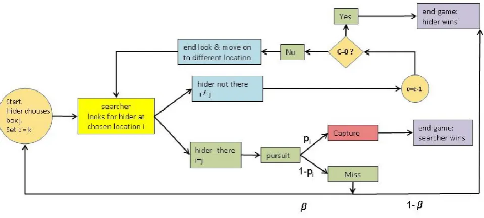
discussed in the previous section: the Hider chooses a location to hide in and the Searcher chooses a subset S of cardinality k to inspect. There is no in‡uence of previous play in earlier stages, except in the variation discussed in the …nal section, where the Hider cannot return to a location where he has previously hidden. There are three possible outcomes:

1. If the Searcher does not …nd the Hider, then the game ends with zero payo¤ for the Searcher and a payo¤ of one to the Hider. (Hider wins.)

2. If the Searcher …nds the Hider and successfully pursues it (captures it), then the game ends with a payo¤ of one to the Searcher and a payo¤ of zero to the Hider. (Searcher wins.)

3. If the Searcher …nds the Hider but does not catch it, then there are two possibilities. With probability 1 the predator gives up and the game ends with a win for the Hider. With the persistence probability the process restarts with the Hider …nding a new location.

1

1:jpg

Figure 1. Flowchart of the repeated game dynamics.

4.2

Basic lemmas for

G

(

k;

)

The basic equation for the valuev of the gameG(k; ), with persistence , will be later

shown to be _n

X

1

v

pi+ (1 pi) v

=k: (6)

Lemma 2 The LHS of (6) is (continuous) strictly monotonic increasing in v: Thus, equation (6) has a unique positive root v; 0< v 1:

Proof. The left hand side (LHS) of equation (6) can be written as

LHS =

n

X

1

1

pi=v+ (1 pi)

so it is a strictly monotonic increasing function ofv forv >0:This function continuously increases from 0 to at least n as v increases from 0 to 1: Since k n; it follows by continuity that there exists a unique root for equation (6).

De…nition 3 Let v1 satisfy

v1 =p1+ (1 p1) v1 (7)

so

v1 =

p1

1 +p1

: (8)

It immediately follows from Lemma 2 that

Lemma 4 As v increases from 0 to v1 , LHS of (6) continuously increases from 0 to

M given by

M =

n

X

1

v1

pi+ (1 pi) v1

=

n

X

1

p1

pi(1 ) +p1

: (9)

Also, as persistence increases from 0 to 1; M increases from

n

P

1

p1=pi to n:

Lemma 5 If k < M; then for any i

v < pi+ (1 pi) v (10)

Proof. By Lemma 4 if k < M; then v < v1 so v < p1+ (1 p1) v: Since the RHS

of (10) is a convex combination of 1,and v 1and pi p1; the result follows.

4.3

Type I solutions of

G

(

k;

)

Theorem 6 (Type I) If k M (see (9)), then the solution of the game G(k; ) is of Type I:

The optimal strategies, unique for k < M; are

h_i = v=k

pi+ (1 pi) v

for the Hider, and (11)

r_i = v

pi+ (1 pi) v

for the Searcher. (12)

The valuev of the game is the unique solution of equation (6), as guaranteed by Lemma 2.

n

X

1

v

pi+ (1 pi) v

=k:

Proof. Assume that k < M: First note that for all i; r_i <1by Lemma 5.

We now show that r = (r₁; :::; r_n) guarantees capture probability equal to v which solves equation (6) against any hiding strategy. For obtaining the minimum probability of capture, achievable by the Hider, if the searcher uses r the Hider has to solve the corresponding Markov Decision Process (MDP) [22] with just two states (a ‘free’state and an absorbing state ‘capture’) and a …nite action space for the Hider. In this MDP there are no costs involved except for a cost 1 which is paid by the Hider if the searcher visits her location (and the process then enters into the absorbing state ‘capture’). By the basic theory of MDP we need to take into account only deterministic stationary strategies for the Hider, i.e., always hiding at the same location, say j: For any such j the probability of capture if the Searcher uses r is

1

X

m=0

r_j (1 pj) m 1

r_jpj =

r_jpj

1 r_j (1 pj)

=v

by (12).

Next we show that h = (h₁; :::; h_n) keeps the probability of capture to at most v against any search strategy. In order to obtain the maximum probability of capture achievable by the searcher if the hider uses h we have to solve an analogous two state MDP for the searcher. Again, we need to consider only deterministic stationary search strategies of searching only a set ofklocations, sayi1; :::; ik:For any such set of locations

the probability of capture if the Hider uses h is calculated as follows. The probability of another round of the process is

B =

k

X

j=1

Thus, the overall probability of capture is 1 X m=0 Bm k X j=1

h_ijpij =

Pk

j=1hijpij

1 B =

Pk j=1

v=k

p_ij+(1 p_ij) vpij

1 Pk_j=1 v=k

p_ij+(1 p_ij) v 1 pij

(14)

by (13) and (11).

In order to calculate (14) observe that for anydj >0; j = 1; : : : ; k;with cj =y(1 dj);

we have _P

jcj=k

1 P_jdj=k

=

y k

P

j(1 dj)

1 k P j1 1 k P

jdj

=y

1

k

P

j(1 dj)

1

k

P

j(1 dj)

!

=y:

Denote now _vp

ij

pij + 1 pij v

=cj

and

1 pij v

pij+ 1 pij v

=dj

then _c

j

1 dj

=v

so the expression given by (14) is equal to v: Thus, the hiding strategy h assures probability of capture at most v given by equation (6). We have thus shown that v is the value of the game and (h ; r ) is a Nash equilibrium.

We next show that r = (r₁; :::; r_n)is the unique search strategy that guarantees the payo¤v given by (6). Assume that there exists a location j withrj < _pj+(1v_{pj) v}: Then

by hiding atj the Hider would make the Searcher’s payo¤ rj[pj + (1 pj) v]< v:

Thus, in order to guarantee payo¤v all ri would have to satisfy

ri

v

pi+ (1 pi) v

:

But r has to satisfy (2) so by (6) and Lemma 2 we must have equality. We have thus proved the uniqueness of r :

We now prove the uniqueness of h :

If

hj >

v=k

then the Searcher can get more than v by using a vector r with ri = (1 )_pi+(1v_{pi) v}

for all i₆=j and rj = _pj+(1v_{pj) v} + P i6=j

v

pi+(1 pi) v , where is a small positive number.

Thus, the payo¤ for the Searcher using R is

(1 )v+

n

X

i=1

v

pi+ (1 pi) v

hj[pj + (1 pj) v]>(1 )v+ n

X

i=1

v

pi+ (1 pi) v

v=k > v:

4.4

Type II solution for general

and

k

M

Here we show that ifk M , whereM is given by (9), then the optimal solution is Type II: always hide at the most favorable location i.e. at location 1 which has the smallest pi:

Theorem 7 (Type II) Suppose k M , where M is given by (9). Then v =v1 given

by (8), and an optimal solution for the Hider is to hide at location 1 (Type II). For the Searcher it is optimal to use an r1 _{vector satisfying}

r1₁ = 1; and

r1_i v1

pi+ (1 pi) v1

for i 2:

Proof. By (7), hiding at location1 guaranteesv1 for the Hider. Also, the vectorr1;

which guarantees v1 against any hiding location, is feasible by (9) which implies that

n

X

i=1

v1

pi+ (1 pi) v1

=M k:

4.5

The ranges of Type I and II solutions

Here we show that in general there is a cuto¤ value of the persistence probability above which the game G(k; ) has only Type I (mixed) solutions and below which it has only Type II (pure) solutions. Sometimes there are only Type I solutions.

Theorem 8 For a given k n; Let k denote the solution of the equation

k =w(p; )

n

X

1

p1

pi(1 ) +p1

: (16)

1. If > _k , then there are only Type I solutions to the game G(k; ): 2. If < _k , then there are only Type II solutions to the gameG(k; )

3. If the equation (16) has no solution, then there are only Type I solutions to the game G(k; ):

Proof. M given by (9) is monotonic increasing with : Thus, > _k implies that k < M: Hence Theorem 6 implies that the unique solution of G(k; ) is of Type I. Similarly < _k implies thatk > M so Theorem 8 implies that the solution of G(k; )

is of Type II.

If (16) has no solution, then it must mean that the right hand side w1 of (16) is always

greater than k (because for = 1 the w1 equals n) so there are always only Type I

solutions to the game G(k; ):

Note that 1 2 ::: n = 1;because the denominator of (9) is decreasing with

:

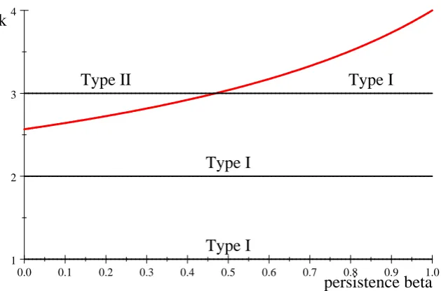
Example 9 In order to illustrate both types of solution for G(k; ), we consider …rst an example with four hiding location and take the capture probability vector to be p = (:2; :3; :4; :5):

0.0 0.1 0.2 0.3 0.4 0.5 0.6 0.7 0.8 0.9 1.0 1

2 3 4

persistence beta k

Type I Type I

Type I Type II

Figure 2. Plot of k=w( ) for capture probabilities p:

Figure 2 shows which strategy type is optimal for p = p: We plot the curve k = w( )

So for example when =:1;Type II strategies are optimal fork >2:6:But askis always an integer in our model (the number of searches), this e¤ectively means that for =:1

Type II strategies are optimal only when k = 3 (or in the trivial case k = 4; where all locations are searched). For k equal to 1 or 2, the …gure shows that Type I strategies are optimal for any persistence probability . If we …x k = 3; the line at height 3 intersects w( ) at about 3 = 0:469, which is thus the cuto¤ value of for Type II strategies and

Type I strategies. That is, when < 0:469 the solution to G(3; ) is of Type II, while for >0:469 the solution is of Type I.

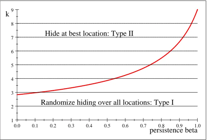
Example 10 We now consider a larger arena with nine hiding locations, with capture probabilities given by the vectorp^= (:1; :2; :3; :4; :5; :6; :7:; :8; :9):Figure 3 plots the curve k = w( ) which again gives the least k; as a real number, for which Type II strategies are optimal. Since in our model k is the integer giving the number of searches, Figure 3 only has implications for integer values of k; which are drawn as horizontal lines. The intersection of the curve w( ) with the horizontal line at height k is called _k; and for

k the solution fork searches is of Type II because there the line of heightk is above

the curve k =w( ): For _k; the solution for k searches is of Type I. Note that for k = 1;2 we only have Type I solutions, but for higher k we have both types.

0.0 0.1 0.2 0.3 0.4 0.5 0.6 0.7 0.8 0.9 1.0 1

2 3 4 5 6 7 8 9

persistence beta k

Hide at best location: Type II

Randomize hiding over all locations: Type I

Figure 3. Plot of k=w( ) for capture probabilitiesp::^

Remark 11 Note that in general if

n

X

1

p1

pi

(or, equivalently, p1 > j ) then G(k; ) has only Type I solutions for all k j: This

follows from Theorem 9 because the RHS of (16) at = 0is greater thenj so no solutions for (16) exist if k j: So for example if p = (0:5; 0:5;1;1) we have equality for j = 3

so we have only Type I solutions for k= 1 and 2; and if k = 3 only Type I solutions for >0:

4.6

An alternative approach to the repeated game

An alternative way of obtaining some of the results about the gameG(k; )is to reduce it to the one stage game by changing the capture probabilities. Suppose the value of the game G(k; ) is known to be some numberv: If the Hider hides at a locationi and the Searcher visits it then the payo¤ to the Searcher can be written as

q=pi+ (1 pi) v;

because the Searcher wins immediately (payo¤ 1) with probabilitypi and with

probabil-ity(1 pi) he gets to play the game (with value v) again. The remaining probability

can be ignored as it gives him payo¤0. It follows that the multi-period game G(k; )

is equivalent to the one stage game ( = 0) with capture probabilitiesqi:

Using (5) of Theorem 1 with qi replacing pi we get the implicit equation

v = min (k ; q1) = min (k ; p1+ (1 p1) v) (17)

where

= _P1₁

qi

.

The implicit equation (17) can be solved by using Lemmas 2 and 4. Solutions with the minimum in the …rst coordinate give Type I solutions and those with the minimum in the second coordinate give Type II solutions.

5

Discussion

We …rst address here the biological signi…cance of our …ndings and end up the paper with an enhancement of our analysis by accounting for the possibility that prey do not return to locations where they were previously found but escaped capture.

beta means prey is more likely to be found –but in this case he is less likely to hide at best location. This implies more randomization, so the e¤ect of more searches due to persistence is the opposite. This can be seen in Figure 3, where increasingk (going up) leads into the type II region whereas increasing beta (going right) leads into the type I region.

Despite extensive search, we were unable to …nd descriptions of biological interactions in which the arena was mapped with su¢ cient precision to identify hiding locations, enabling us to test the predictions of the model. In the only case for which we have su¢ cient information, the leafminer case detailed in the introduction, the very large number of ovipositor insertions leads to a full randomization of the ‡eeing locations of the caterpillar location (see [18] and [19]). By contrast, there is ample evidence that persistence of attacks leads to increased randomness in other characteristics of prey escape for several biological systems [23]. For example, the distribution of angle of ‡eeing in cockroaches increases in variance with an increasing degree of persistence of attacks [23]. In all cases, increasing randomness in prey escape hampers any learning process in the persistent predator.

search and attack.

5.1

Improving the realism of the repeated search model

Our model includes two assumptions that might be relaxed. The …rst is that the available hiding locations do not change over time and the second is that once the prey successfully evades the predator, he will not be captured before he …nds a new hiding location.

Up to now we have been assuming that in the multi stage games the available hiding locations remain the same over time. However we now consider the implications of the opposite assumption, namely that if the prey successfully escapes after being found at location j; he may not return to that location in the next stage game. This restriction on prey strategies is in accordance with two biological examples from the introduction: a wary seal might prefer to swim to a di¤erent breathing hole and a wary caterpillar might have jerked in its mine and relocated itself somewhere else. As this restriction is a complicating feature, we explore the consequences of the ‘no return’ assumption in the simplest setting, a two stage game four locations with full persistence = 1 in the …rst stage. We consider the example where the capture probability vector is p = (:2; :3; :4; :5):In the version with the no-return assumption, the optimal hiding strategy in stage 1 is given by ^h= (0:331;0:268;0:218;0:183):In the unrestricted version (where the hider can return to a previously occupied location) the optimal hiding strategy in stage 1 is given by ~h= (0:355;0:263;0:209;0:173):Note that when return is prohibited, the optimal probability of hiding at the best location, location 1; goes down from:355

(in the unrestricted case) to :331: The intuition for this decreased probability is that hiding at location1in the …rst stage now has the disadvantage that this good location is no longer available in the second stage. Of course if the probability of hiding at location

1 goes down, this must be compensated by increasing some of the other probabilities. But it is interesting to note, in this respect, that the ratios ^hi=~hi form an increasing

sequence, (0:931;1:018;1:046;1:058). In terms of the value (probability that predator wins), it goes up from ~v = (~q) = :093 in the unrestricted game to v^ = (^q) = :100

in the game where the prey is restricted to no-return strategies. Of course it is well known that, in zero sum games, restricting the strategies of one player results in a lower expected payo¤ for that player, so the direction of change is not surprising.

The second assumption that might be relaxed concerns the ability of the prey to safely reach any new hiding location once he has escaped pursuit by the predator at location i:This models the situation where the prey is only vulnerable to capture while in one of the hiding locations (perhaps these are places to feed and out in the open). This is the same as in the model of [10]. However it is possible in theory to incorporate a probabilitypij that the prey will be captured when changing from locationito locationj:

This could model the cover in the region between the hiding locations. Clearly locations i where the numbers pij and pji are high would then become less attractive to hide at.

hiding locations, so that if hiding in location i in one period the prey could only move to an adjacent location i0 _{in the next period.}

Both these altered models could be investigated in future research, and we thank an anonymous referee for suggesting modi…cations of our model in such directions.

5.2

Conclusion

This work is the …rst to extend search games to repeated games. It thus expands greatly the number of observed searcher-hider interactions played repeatedly by the same pair of agents in the same environment and also highlights the opposite inferences drawn when incorporating multiple bouts of search and escape, in comparison with the ones obtained in one stage games. Our next goal is to further increase the realism of search games by developing stochastic search games to deal with the giving up time of persistent, learning predators.

6

Acknowledgements

We thank I. Stirling and A. Derocher for sharing their insights on polar bear attacks on seals and two referees for insightful comments. Steve Alpern wishes to thank the Air Force O¢ ce of Scienti…c Research (grant FA9550-14-1-0049).

References

[1] Davies, N.B., Krebs, J.R. & West, S.A. (2012). An introduction to Behavioral Ecology. 4th edition. Wiley, New York.

[2] Stephens, D.W., Krebs, J.R. (1986). Foraging theory. Princeton University Press, New Jersey.

[3] Gal, S., & Casas, J. (2014). Succession of hide–seek and pursuit–evasion at hetero-geneous locations. Journal of The Royal Society Interface 11(94), 20140062. [4] Morice S., Pincebourde S., Darboux F., Kaiser W., Casas J. (2013). Predator–prey

pursuit–evasion games in structurally complex environments. Integr. Comp. Biol. 53, 767–779. (doi:10.1093/icb/ict061)

[5] Alpern S, Gal S. (2003). The Theory of Search Games and Rendezvous. Dordrecht, The Netherlands: Kluwer Academic Publishers.

[7] Alpern, S., Fokkink, R., Gal, S., & Timmer, M. (2013). On search games that include ambush.SIAM Journal on Control and Optimization 51(6), 4544-4556. [8] Alpern, S., Fokkink, R., Lidbetter, T., N. Clayton, N. (2012). A search game model

of the scatter hoarder’s problem. Journal of the Royal Society. Interface 9 (2012): 869-879.

[9] Zoroa N, Fernndez-Sez MJ, Zoroa P. 2011 A foraging problem: sit-and-wait versus active predation. Eur. J. Oper. Res. 208, 131–141. (doi:10.1016/j.ejor.2010.08.001) [10] Zoroa, N., Fernández-Sáez, M. J., & Zoroa, P. (2014). Ambush and Active Search

in Multistage Predator–Prey Interactions.Journal of Optimization Theory and Ap-plications, 1-18.

[11] Arcullus, R. (2013). A discrete search-ambush game with a silent predator.In Search Theory. A Game Theoretic Perspective (pp. 249-266). Springer New York.

[12] Broom, M. (2013). Interactions Between Searching Predators and Hidden Prey. In Search Theory. A Game Theoretic Perspective (pp. 233-248). Springer New York. [13] Pitchford, J. (2013). Applications of Search in Biology: Some Open Problems. In

Search Theory: A Game Theoretic Perspective (pp. 295-303). Springer New York. [14] Cooper Jr, W. E. & Blumstein, D.T. (2015). Escaping from predators: an

integra-tive view of escape decisions. Cambridge University Press.

[15] Rudebeck, G. (1951). The choice of prey and modes of hunting of predatory birds with special reference to their selective e¤ect. Oikos, 3(2), 200-231.

[16] Martin, J., & Lopez, P. (2003). Changes in the escape responses of the lizard Acan-thodactylus erythrurus under persistent predatory attacks. Copeia, (2), 408-413. [17] Bateman, P. W., & Fleming, P. A. (2014). Switching to Plan B: changes in the

escape tactics of two grasshopper species (Acrididae: Orthoptera) in response to repeated predatory approaches. Behavioral ecology and sociobiology, 68(3), 457-465. [18] Meyhöfer, R., Casas, J., & Dorn, S. (1997). Vibration–mediated interactions in a host–parasitoid system. Proceedings of the Royal Society of London B: Biological Sciences, 264(1379), 261-266.

[19] Djemai, I., Casas, J., & Magal, C. (2004). Parasitoid foraging decisions mediated by arti…cial vibrations. Animal Behaviour, 67(3), 567-571.

[21] Selten, R. (1980). A note on evolutionarily stable strategies in asymmetric animal con‡icts.Journal of Theoretical Biology 84 (1), 93–101.

[22] Puterman. M. L. (1994). Markov Decision Processes: Discrete Stochastic Dynamic Programming. John Wiley & Sons, Inc., New York, NY, USA.

[23] Domenici, P., Blagburn, J. M., & Bacon, J. P. (2011). Animal escapology I: theoret-ical issues and emerging trends in escape trajectories. The Journal of experimental biology, 214(15), 2463-2473.

[24] Stirling, I. (1974). Midsummer observations on the behavior of wild polar bears (Ursus maritimus). Canadian Journal of Zoology, 52(9), 1191-1198.

[25] Hall, C. F. (1864). Life with the Esquimaux, 2 vols. London: Sampson, Low, Son, and Marston.