Stability and time delay tolerance analysis approach for networked control systems

warwick.ac.uk/lib-publications

Original citation:

Khalil, Ashraf F. and Wang, Jihong. (2015) Stability and time delay tolerance analysis

approach for networked control systems. Mathematical Problems in Engineering, 2015. pp.

1-9. 812070.

Permanent WRAP URL:

http://wrap.warwick.ac.uk/78883

Copyright and reuse:

The Warwick Research Archive Portal (WRAP) makes this work of researchers of the

University of Warwick available open access under the following conditions.

This article is made available under the Creative Commons Attribution 4.0 International

license (CC BY 4.0) and may be reused according to the conditions of the license. For more

details see:

http://creativecommons.org/licenses/by/4.0/

A note on versions:

The version presented in WRAP is the published version, or, version of record, and may be

cited as it appears here.

Research Article

Stability and Time Delay Tolerance Analysis Approach for

Networked Control Systems

Ashraf F. Khalil

and Jihong Wang

1_{Electrical and Electronic Engineering Department, University of Benghazi, Benghazi, Libya} 2_{School of Engineering, University of Warwick, Coventry CV4 7AL, UK}

Correspondence should be addressed to Ashraf F. Khalil; ashraf.khalil@uob.edu.ly

Received 9 August 2014; Revised 27 October 2014; Accepted 29 October 2014

Academic Editor: Yun-Bo Zhao

Copyright © 2015 A. F. Khalil and J. Wang. This is an open access article distributed under the Creative Commons Attribution License, which permits unrestricted use, distribution, and reproduction in any medium, provided the original work is properly cited.

Networked control system is a research area where the theory is behind practice. Closing the feedback loop through shared network induces time delay and some of the data could be lost. So the network induced time delay and data loss are inevitable in networked control Systems. The time delay may degrade the performance of control systems or even worse lead to system instability. Once the structure of a networked control system is confirmed, it is essential to identify the maximum time delay allowed for maintaining the system stability which, in turn, is also associated with the process of controller design. Some studies reported methods for estimating the maximum time delay allowed for maintaining system stability; however, most of the reported methods are normally overcomplicated for practical applications. A method based on the finite difference approximation is proposed in this paper for estimating the maximum time delay tolerance, which has a simple structure and is easy to apply.

1. Introduction

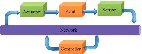
The key feature of networked control systems (NCSs) is that the information is exchanged through a network among control system components. So the network induced time delay is inevitable in NCSs. The time delay, either constant (up to jitter) or random, may degrade the performance of control systems and even destabilize the systems. NCSs can be defined as a control system where the control loop is closed through a real-time communication network [1]. The term networked control systems first appeared in Walsh’s article in 1999 [2]. A typical organization of an NCS is shown in Figure 1. The reference input, plant output, and control input are exchanged through a real-time communication network. The main advantages of NCSs are modularity, simplified wiring, low cost, reduced weight, decentralization of control, integrated diagnosis, simple installation, quick and easy maintenance [3], and flexible expandability (easy to add/remove sensors, actuators, or controllers with low cost). NCSs are able to easily fuse global information to make intelligent decisions over large physical spaces which is important for many engineering systems such as the power system.

As the control loop is closed through a communication network the time delay and data dropout are unavoidable. Therefore networked control system can be regarded as a special case time delay system and many authors applied the time delay theorems to study NCSs [4]. Time delay, no doubt, increases complexity in analysis and design of NCSs. Conventional control theories built on a number of standing assumptions including synchronized control and nondelayed sensing and actuation must be reevaluated before they can be applied for NCSs [5].

The main goal of the most recent work is to reduce the conservativeness of the maximum time delay by using Lyapunov-Krasovskii functional with improved algorithms for solving the linear matrix inequalities (LMIs) set but with the expense of increasing complexity and computation time. Analytical and graphical methods have been studied in the literature (see, e.g., [6]). The stability criteria for NCSs based on Lyapunov-Krasovskii functional approach have been reported in [7–9]. In [7], a Lyapunov-Krasovskii function is used to derive a set of LMIs and the stability problem is generalized to a feasibility problem for the LMIs set. In many of the previously reported works, the controller is

Plant

Actuator Sensor

Controller Network

Figure 1: A typical networked control system.

designed in the absence of the time delay. In [10], an improved Lyapunov-Krasovskii function is used with triple integral terms. The LMI methods require the closed-loop system to be Hurwitz [8,11,12]. In [13], a modified cone complementary linearization algorithm based on the Lyapunov-Krasovskii approach is implemented. And the method reported in [14] is claimed to be less conservative and the computational complexity is reduced.

The authors in [15] derived an LMI-based method in the frequency domain, and then the LMI is transformed onto an equivalent nonfrequency domain LMI by applying Kalman-Yakubovich-Popov lemma. It has been reported in [16] that the ordinary Lyapunov stability analysis is linked by a suggested variable to state vectors through convolution and the stability analysis is simplified to only require solving a nonlinear algebraic matrix equation.

In [11], the hybrid system technique is used to derive a stability region. An upper bound is derived for time delay in an inequality form and the results are rather conservative. The hybrid system stability analysis technique has also been used in [17]. A simple analytical relation is derived between the sampling period, the time delay, and the controller gains. The same approach is used in [18] with more conservative stability region results. The model-based approach for deriving neces-sary and sufficient conditions for stability is presented in [19]. The stability criteria are derived in terms of the update time and the parameters of the model. The model-based approach is then extended to multiunits NCS in [20]. The optimal stochastic control was studied in [21] with a discrete-time system model where the random time delays are modeled using Markov chains and the controller uses the knowledge of the past state time delays by time stamping.

Most of the previously developed approaches require excessive load of computations, and also, for higher order systems, the load of computations will increase dramatically. In practice, engineers may find it difficult to apply those available methods in control system design because of the complexity of the methods and lack of guideline in linking between the design parameters and the system performance. Almost all the design procedures highly depend on the postdesign simulation to determine the design parameters. So there is a demand for a simple design approach with clear guidance for practical applications. In this paper, a new stability analysis and control design method is proposed, in which the design approach is simple and a clear design procedure is given.

The paper starts from the mathematical model of NCS and then the proposed method for estimating the maximum allowable delay bound is briefly described. A few examples are illustrated and the results are compared with those previously published in the literature. The cart and inverted pendulum problem is used to study the effect of the parameters on the maximum allowable delay bound.

2. Mathematical Analysis

Although the issues involved with time delays in control systems have been studied for a long time, it is difficult to find a method simple enough to be accepted by control system design engineers. It is found that the most previously reported methods rely on LMI techniques and they are generally too complicated for practical engineers to use and also involve heavy load of numerical calculations and computing time. The paper proposes a new method which has a simple structure and is used for estimating the maximum time delay allowed while the system stability can still be maintained. In most control systems the sampling time is preferred to be small [22]. The maximum allowable delay bound (MADB) can be defined as the maximum sampling period that guarantees the stability even with poor system performance. A continuous time-invariant linear system is shown inFigure 2and given by

̇

x(𝑡) =Ax(𝑡) +Bu(𝑡) ,

y(𝑡) =Cx(𝑡) +Du(𝑡) , (1)

wherex(𝑡) ∈R𝑛is the system state vector,u(𝑡) ∈R𝑚is the system control input,y(𝑡) ∈ R𝑝 is the system output, and

A∈R𝑛×𝑛_,B∈R𝑛×𝑚_,C∈R𝑝×𝑛_{, andD∈R}𝑝×𝑚_{are constant}

matrices with appropriate sizes.

Suppose that the control signals are connected to the control plant through a kind of network, so the time delay is inevitable to be involved in the feedback loop. The state feedback is therefore can be written as

u(𝑡) =Kx(𝑡 − 𝜏_𝑠𝑐− 𝜏_𝑐− 𝜏_𝑐𝑎) , (2)

where 𝜏_𝑠𝑐 is the time delay between the sensor and the controller,𝜏_𝑐is the time delay in the controller, and𝜏_𝑐𝑎is the time delay from the controller to the actuator.K represents the feedback control gains with appropriate size. From(2)the networked control system can be modeled where the time delay is lumped between the sensor and the controller as shown inFigure 3.

The time delay may be constant, variable, or even random. In NCSs, the time delay is composed of the time delay from sensors to controllers, time delay in the controller, and controllers to actuators time delay which is given by

𝜏 = 𝜏_𝑠𝑐+ 𝜏_𝑐+ 𝜏_𝑐𝑎. (3)

For a general formulation the packet dropouts can be incor-porated in(3)as follows:

Mathematical Problems in Engineering 3

Actuator Plant Sensor

Controller

𝜏ca 𝜏sc

x(t)

Kx(t − 𝜏sc− 𝜏c− 𝜏ca)

Kx(t − 𝜏sc− 𝜏c) _{x(t − 𝜏sc)}

Figure 2: A networked control system with the time delay both from the sensor to the controller and from the controller to the actuator.

Actuator Plant Sensor

Controller

𝜏ca+ 𝜏sc

x(t)

Kx(t − 𝜏sc− 𝜏c− 𝜏ca)

x(t − 𝜏sc− 𝜏ca)

Figure 3: A simplified model of the networked control system.

where𝑑is the number of dropouts andℎthe sampling period. And by(4)the data dropouts can be considered as a special case of time delay [23,24]. It is supposed that the following hypotheses hold.

Hypothesis 1(H.1). (i) The sensors are clock driven. (ii) The controllers and the actuators are event driven. (iii) The data are transmitted as a single packet. (iv) The old packets are discarded. (v) All the states are available for measurements and hence for transmission.

Hypothesis 2(H.2). The time delay𝜏is small to be less than one unit of its measurement.

Definition 1(D.1). For a function𝑓(𝑡), the𝑛th order reminder for its Taylor’s series expansion is defined by

𝑅_𝑛(𝑓 (𝑡) , 𝜏) =∑∞

𝑛

𝑓(𝑛)(𝜉)

𝑛! 𝜏𝑛. (5)

Applying the state feedback proposed in(2)to the system(1), we have

̇

x(𝑡) = Αx(𝑡) +BKx(𝑡 − 𝜏) . (6)

From(6), the following can be derived:

̇

x(𝑡) = (A+BK)x(𝑡) +BK[x(𝑡 − 𝜏) −x(𝑡)] . (7)

Theorem 2. Suppose that (H.1) and (H.2) hold. For system(1)

with the feedback control of(2), the closed-loop system is glob-ally asymptoticglob-ally stable if𝜆_𝑖(Ψ) ∈ 𝐶−, for𝑖 = 1, 2, . . . , 𝑛and all the state variables’ 2nd order reminders are small enough for the given value of𝜏, whereΨis given by

Ψ = [(𝐼 + 𝜏BK)−1(A+BK)] . (8)

Proof. The expression forx(𝑡 − 𝜏)can be obtained by Taylor expansion as

x(𝑡 − 𝜏) =∑∞

𝑛=0(−1)

𝑛 𝜏𝑛

𝑛!x(𝑛)(𝑡) , (9)

where x(𝑛)(𝑡) is the 𝑛th order derivative. The first order approximation of the delay term is given by

x(𝑡 − 𝜏) =x(𝑡) − 𝜏 ̇x(𝑡) + (𝜏2

2) ̈x(𝑡) +R3(x, 𝜏) ,

x(𝑡 − 𝜏) ≈x(𝑡) − 𝜏 ̇x(𝑡) + (𝜏2

2) ̈x(𝑡) ,

x(𝑡 − 𝜏) =x(𝑡) − 𝜏 ̇x(𝑡) +R2(x, 𝜏) .

(10)

From(10)it can be seen thatR₂(𝑥, 𝜏)depends on the time delay,𝜏, and the higher order derivatives ofx(𝑡)which can be neglected if the time delay and the norm ofR₂(𝑥, 𝜏)are small. Then we have

x(𝑡 − 𝜏) ≈x(𝑡) − 𝜏 ̇x(𝑡) . (11)

The assumption in (11) can be used without significant error, and this can be true for the following reasons. Firstly, the time delay in a computer network is very small in order of milli- or microseconds and at the worst few tenths of the second. Secondly, in most of the real control system applications the linearized model is used and the higher order terms are already neglected. Additionally, the higher order derivatives will be multiplied by𝜏𝑛/𝑛which is much more smaller than𝜏because𝜏 ≪ 1. Substituting(11)into(7), the following can be derived:

̇

x(𝑡) ≈ (A+BK)x(𝑡) − 𝜏BKẋ(𝑡) , (12)

̇

x(𝑡) ≈ [(I+ 𝜏BK)−1(A+BK)]x(𝑡) , (13)

Ψ = [(I+ 𝜏BK)−1(A+BK)] . (14)

The system(13)will be globally asymptotically stable if

𝜆𝑖(Ψ) ∈C−, for𝑖 = 1, 2, . . . , 𝑛. (15)

Corollary 3. Suppose (H.1) and (H.2) hold. For the control

system(1)with the control law(2), the closed-loop system is globally asymptotically stable if

𝜏 < 1

‖BK‖. (16)

Proof. For system (1), suppose that the state feedback has been designed to ensure𝜆(A+BK) ∈ C−. Therefore, for a chosen positive definite matrixP=PT, it will find a positive definite matrixQ=QTto have

Choose a Lyapunov functional candidate as

V(𝑥) =xTPx> 0 ∀x ̸=0. (18)

The objective for the next step is to find the range of𝜏that will ensure (V̇(𝑥) < 0 ∀x ̸=0) [25–27]. Taking the derivative of(18),

̇

V(𝑥) = ̇xTPx+xTPẋ

≈xT[(A+BK)TPP−1(I+ 𝜏BK)−TP

+P(I+ 𝜏BK)−1P−1P(A+BK)]x

−xT[P(A+BK) + (A+BK)TP]x

+xT[P(A+BK) + (A+BK)TP]x

≈xT[(A+BK)TPP−1(I+ 𝜏BK)−TP

− (A+BK)TP+P(I+ 𝜏BK)−1P−1P(A+BK)

− P(A+BK) ]x−xTQx.

(19) Rearranging the terms in the above equation, then

̇

V(x) ≈xT{(A+BK)TP[P−1(I+ 𝜏BK)−TP−I]

+ [P(I+ 𝜏BK)−1P−1−I]P(A+BK)}x

−xTQx.

(20)

IfP(I+ 𝜏BK)−1P−1−I=I then(20)will become

xT[P(A+BK) + (A+BK)TP]x−xTQx= 0. (21)

Move the last term to the right hand side; the following will be derived:

xT[P(A+BK) + (A+BK)TP]x=xTQx. (22)

So‖P(A+BK) + (A+BK)TP‖ ⋅ ‖x‖2= ‖Q‖ ⋅ ‖x‖2.

Assuming that we can find a positive number to make the following hold:

󵄩󵄩󵄩󵄩

󵄩P(A+BK) + (A+BK)TP󵄩 = 2𝛾󵄩󵄩󵄩󵄩 󵄩󵄩󵄩󵄩󵄩(A+BK)TP󵄩󵄩󵄩󵄩󵄩 = ‖Q‖

(23)

then𝛾can be considered as the norm ofP−1(I+ 𝜏BK)−1P−I. Therefore, we have

xT[(A+BK)TP[P−1(I+ 𝜏BK)−TP−I]

+ [P(I+ 𝜏BK)−1P−1−I]P(A+BK)]x

≤ 2 󵄩󵄩󵄩󵄩󵄩(P−1(I+ 𝜏BK)−TP−I)P(A+BK)󵄩󵄩󵄩󵄩_{󵄩 ⋅ ‖}x‖2.

(24)

Choose

󵄩󵄩󵄩󵄩

󵄩P−1(I+ 𝜏BK)−1P−I󵄩󵄩󵄩󵄩󵄩 ≤ 1. (25)

Use Neumann series formula for the inverse of the sum of two matrices:

(I+ 𝜏BK)−1

=I− 𝜏BK+ 𝜏2(BK)2− 𝜏3(BK)3+ ⋅ ⋅ ⋅ − . (26)

For small time delays𝜏 ≪ 1(26)can be given as

(I+ 𝜏BK)−1_{≈I− 𝜏BK. (27)}

Applying(27)into(25)then we have

󵄩󵄩󵄩󵄩

󵄩P−1(I+ 𝜏BK)−1P−I󵄩󵄩󵄩󵄩󵄩

≈ 󵄩󵄩󵄩󵄩󵄩P−1_{(I− 𝜏BK)P−I}󵄩󵄩󵄩󵄩

󵄩 = ‖𝜏BK‖ < 1.

(28)

And finally we get

𝜏 < _‖BK‖1 . (29)

That is, for any𝜏 < 1/‖BK‖,V̇(𝑥) < 0, the system will be globally asymptotically stable.

Theorem 2 and Corollary 3 give us a simple tool in estimating the maximum allowable time delay for NCSs. Further analysis in the frequency domain is described below. Taking Laplace transform of(12), we have

𝑠X(𝑠) = (A+BK)X(𝑠) − 𝜏𝑠BKX(𝑠) ,

[𝑠I− (A+BK) + 𝜏𝑠BK]X(𝑠) = 0. (30)

The characteristics equation is defined as

[𝑠I− (A+BK) + 𝜏𝑠BK] = 0. (31)

For a stable system the roots of the characteristics equation

(31) must lie in the left hand side of the 𝑠-plane. From the characteristics equation, it is clear that the term𝜏𝑠BK influences the system performance and the stability as the term of𝜏𝑠BK may push the closed-loop system poles toward the right hand side of the𝑠-plane.

As we have seen the system characteristic is determined by the term 𝜏BKx(𝑡)̇ in a certain level. This term can be regarded as a differentiator in the feedback loop, so it will introduce extra zeros to the closed-loop system and the time delay can be considered to have resulted in a variable gain to the feedback path. For more accurate estimation the second or third-order difference approximation can be used as follows:

[𝑠I− (A+BK) + 𝜏𝑠BK−𝜏2𝑠2

2 BK] = 0,

[𝑠I− (A+BK) + 𝜏𝑠BK−𝜏2𝑠2

2 BK+

𝜏3_𝑠3

6 BK] = 0.

(32)

Mathematical Problems in Engineering 5

Corollary 4. Suppose that (H.1) and (H.2) hold. The system(2)

with the controller(3)is asymptotically stable if

𝜏 < _{󵄨󵄨󵄨󵄨𝜆} 1

min(BK)󵄨󵄨󵄨󵄨. (33)

Proof. The main assumption is that the eigenvalues of the compensator,BK, are all negative,𝑠₁ < 0, . . . , 𝑠_𝑛 < 0, and are given by

BK− 𝑠I_𝑛×𝑛=[[[_[

[

𝑎₁₁− 𝑠 𝑎₁₂ ⋅ ⋅ ⋅ 𝑎_1𝑛

𝑎₂₁ 𝑎₂₂− 𝑠 ⋅ ⋅ ⋅ 𝑎_2𝑛

... ... d ...

𝑎_𝑛1 𝑎_𝑛2 ⋅ ⋅ ⋅ 𝑎_𝑛𝑛− 𝑠

] ] ] ] ] . (34)

The characteristic equation is the determinant of(34). As-sume that the eigenvalues are given by

𝑠₁= 𝛼₁, . . . , 𝑠_𝑛= 𝛼_𝑛,

𝛼₁< 0, . . . , 𝛼_𝑛< 0. (35)

Preliminary 1 (inverse eigenvalues theorem [28]). Given a matrixX that is nonsingular, with eigenvalues𝜆₁, . . . , 𝜆_𝑛 >

0, 𝜆₁, . . . , 𝜆_𝑛are eigenvalues ofX if and only if𝜆₁−1, . . . , 𝜆_𝑛−1

are eigenvalues ofX−1.

The eigenvalues of(I_𝑛×𝑛+ 𝜏BK)are given by

𝜏 ⋅BK+I𝑛×𝑛− 𝜆I𝑛×𝑛

=[[[_[

[

𝜏𝑎₁₁+ 1 − 𝜆 𝜏𝑎₁₂ ⋅ ⋅ ⋅ 𝜏𝑎_1𝑛

𝜏𝑎₂₁ 𝜏𝑎₂₂+ 1 − 𝜆 ⋅ ⋅ ⋅ 𝜏𝑎_2𝑛

... ... d ...

𝜏𝑎_𝑛1 𝜏𝑎_𝑛2 ⋅ ⋅ ⋅ 𝜏𝑎_𝑛𝑛+ 1 − 𝜆

] ] ] ] ] , (36)

Δ (𝜏 ⋅BK+I_𝑛×𝑛− 𝜆I_𝑛×𝑛)

=det(

[ [ [ [ [

𝜏𝑎₁₁+ 1 − 𝜆 𝜏𝑎₁₂ ⋅ ⋅ ⋅ 𝜏𝑎_1𝑛

𝜏𝑎₂₁ 𝜏𝑎₂₂+ 1 − 𝜆 ⋅ ⋅ ⋅ 𝜏𝑎_2𝑛

... ... d ...

𝜏𝑎𝑛1 𝜏𝑎𝑛2 ⋅ ⋅ ⋅ 𝜏𝑎𝑛𝑛+ 1 − 𝜆

] ] ] ] ] ) ,

Δ (𝜏 ⋅BK+I_𝑛×𝑛− 𝜆I_𝑛×𝑛)

= 𝜏𝑛det((₍

( [ [ [ [ [ [ [ [ [ [

𝑎₁₁+1 − 𝜆

𝜏 𝑎12 ⋅ ⋅ ⋅ 𝑎1𝑛

𝑎₂₁ 𝑎₂₂+1 − 𝜆

𝜏 ⋅ ⋅ ⋅ 𝑎2𝑛

... ... d ...

𝑎_𝑛1 𝑎_𝑛2 ⋅ ⋅ ⋅ 𝑎_𝑛𝑛+1 − 𝜆_𝜏

] ] ] ] ] ] ] ] ] ] ) ) ) ) . (37) Replacing(1 − 𝜆)/𝜏by−𝑠in(37)we get

= 𝜏𝑛det(

[ [ [ [ [

𝑎₁₁− 𝑠 𝑎₁₂ ⋅ ⋅ ⋅ 𝑎_1𝑛

𝑎₂₁ 𝑎₂₂− 𝑠 ⋅ ⋅ ⋅ 𝑎_2𝑛

... ... d ...

𝑎_𝑛1 𝑎_𝑛2 ⋅ ⋅ ⋅ 𝑎_𝑛𝑛− 𝑠

] ] ] ] ]

) = 0. (38)

Solving(38)the eigenvalues are given as

(𝜆₁− 1)

𝜏 = 𝛼1, . . . ,(𝜆𝑛_𝜏− 1) = 𝛼𝑛,

𝛼₁< 0, . . . , 𝛼_𝑛< 0,

𝜆₁= 1 + 𝜏𝛼₁, . . . , 𝜆_𝑛= 1 + 𝜏𝛼_𝑛,

𝛼₁< 0, . . . , 𝛼_𝑛 < 0.

(39)

If𝜏 < 1/|𝛼_max|then all the eigenvalues are positive and the

system is asymptotically stable, and if𝜏 > 1/|𝛼_max|at least one of the eigenvalues will be negative then.

If𝜏 < 1/|𝜆_min(BK)|and (H.1) and (H.2) hold then the

system is asymptotically stable.

Corollary 5. Suppose that (H.1) and (H.2) hold. For system

(1)with the control law(2), the closed-loop system is globally asymptotically stable if

𝜏 < 1

𝑎𝑏𝑠 (KB) (𝑤ℎ𝑒𝑟𝑒 𝑎𝑏𝑠 𝑖𝑠 𝑡ℎ𝑒 𝑎𝑏𝑠𝑜𝑙𝑢𝑡𝑒 V𝑎𝑙𝑢𝑒) . (40)

From Preliminary 1, the signs of the eigenvalues of (I_𝑛×𝑛 +

𝜏BK)−1 and(I_𝑛×𝑛 + 𝜏BK)are the same. For a

single-input-single-output control system the matrixBKcan be written as

BK=[[[_[

[ 𝑏1 𝑏2 ... 𝑏_𝑛 ] ] ] ] ]

[𝑘1 𝑘2 ⋅ ⋅ ⋅ 𝑘𝑛] =

[ [ [ [ [

𝑏1𝑘1 𝑏1𝑘2 ⋅ ⋅ ⋅ 𝑏1𝑘𝑛

𝑏2𝑘1 𝑏2𝑘2 ⋅ ⋅ ⋅ 𝑏2𝑘𝑛

... ... d ...

𝑏_𝑛𝑘₁ 𝑏_𝑛𝑘₂ ⋅ ⋅ ⋅ 𝑏_𝑛𝑘_𝑛

] ] ] ] ] . (41)

The interesting property ofBKis that it is singular. The eigen-values ofBKare given by

BK− 𝜆I_𝑛×𝑛=

[ [ [ [ [ [ [

𝑏₁𝑘₁− 𝜆 𝑏₁𝑘₂ ⋅ ⋅ ⋅ 𝑏₁𝑘_𝑛

𝑏₂𝑘₁ 𝑏₂𝑘₂− 𝜆 ⋅ ⋅ ⋅ 𝑏₂𝑘_𝑛

... ... d ...

𝑏_𝑛𝑘₁ 𝑏_𝑛𝑘₂ ⋅ ⋅ ⋅ 𝑏_𝑛𝑘_𝑛− 𝜆

] ] ] ] ] ] ] . (42)

The characteristics equation ofBKis the determinant of(42)

and is given by

𝜆2−Tr(BK) 𝜆 +1

2[Tr(BK2) −Tr(BK)2]

...

𝜆𝑛−Tr(BK) 𝜆𝑛−1+1

2[Tr(BK2) −Tr(BK)2] 𝜆𝑛−2

+ ⋅ ⋅ ⋅ + 1

2[Tr(BK2) −Tr(BK)2] .

(43)

BecauseBKis singulardet(BK) = 0and hence

det(BK) = 1

2[Tr(BK2) −Tr(BK)2] = 0,

Tr(BK2) =Tr(BK)2.

Substituting(44)into(43), then(43)becomes

𝜆2−Tr(BK) 𝜆 󳨀→ 𝜆 (𝜆 −Tr(BK))

...

(−1)𝑛𝜆𝑛−Tr(BK) 𝜆𝑛−1󳨀→ (−1)𝑛𝜆𝑛−1(𝜆 −Tr(BK)) .

(45)

Finally the eigenvalues ofBKare

𝜆₁, . . . , 𝜆_𝑛−1= 0 𝜆_𝑛=Tr(BK) < 0. (46)

Equation (46) shows that the minimum eigenvalue of BK equalsTr(BK). If the eigenvalues of(I_𝑛×𝑛+ 𝜏BK)are𝑠₁, . . . , 𝑠_𝑛, then the eigenvalues of(I_𝑛×𝑛+ 𝜏BK)−1are1/𝑠₁, . . . , 1/𝑠_𝑛. The eigenvalues of(I_𝑛×𝑛+ 𝜏BK)are given by

𝜏 ⋅BK+I_𝑛×𝑛− 𝑠I_𝑛×𝑛

= [ [ [ [ [ [ [

𝜏𝑏1𝑘1+ 1 − 𝑠 𝜏𝑏1𝑘2 ⋅ ⋅ ⋅ 𝜏𝑏1𝑘𝑛

𝜏𝑏₂𝑘₁ 𝜏𝑏₂𝑘₂+ 1 − 𝑠 ⋅ ⋅ ⋅ 𝜏𝑏₂𝑘_𝑛

... ... d ...

𝜏𝑏_𝑛𝑘₁ 𝜏𝑏_𝑛𝑘₂ ⋅ ⋅ ⋅ 𝜏𝑏_𝑛𝑘_𝑛+ 1 − 𝑠

] ] ] ] ] ] ] .

(47)

By solving(47)it can be found that

𝑠₁, . . . , 𝑠_𝑛−1= 1,

𝑠_𝑛 = 1 + 𝜏 ⋅Tr(BK) = 1 + 𝜏 ⋅ 𝜆_max(BK) (48)

if𝜏 < 1/|Tr(BK)| → 𝑠_𝑛> 0 → 𝑠₁, . . . , 𝑠_𝑛> 0.

For single-input-single-output NCS we have

𝑎𝑏𝑠 (KB) =Tr(BK) ; 𝑡ℎ𝑒𝑛 (49)

if𝜏 < 1/|KB|and both (H.1) and (H.2) hold then the system is

asymptotically stable.

This inequality can be used as a simple and fast tool for estimating the MADB in NCS and involves only single calculation.

3. Stability Analysis Case Studies

In general, two approaches are applied to controller design for NCSs. The first approach is to design a controller without considering time delay and then to design a communication protocol that minimizes the effects caused by time delays. The second approach is to design the controller while taking the time delay and data dropouts into account [11,29]. The proposed method in this paper is used to estimate the MADB for predesigned control system. In this section, a number of examples are studied to demonstrate the proposed method and compare its results with the previously published cases in the literature. In particular, the results derived using the method proposed in this paper have been compared with the results using the LMI method given in [7] and with the fourth-order Pade approximation. The fourth-order Pade approximation [6] is used for the delay term in the𝑠-domain and is defined as

𝑒−𝜏𝑠≈ 𝑃_𝑑(𝑠) = 𝑁_𝐷𝑑(𝑠)

𝑑(𝑠) =

(∑𝑛_𝑘=0(−1)𝑘𝑐_𝑘𝜏𝑘_𝑠𝑘₎

(∑𝑛_𝑘=0𝑐_𝑘𝜏𝑘_𝑠𝑘₎ . (50)

The coefficients are given by

𝑐_𝑘= ((2𝑛 − 𝑘)!𝑛!)

(2𝑛!𝑘! (𝑛 − 𝑘)!) 𝑘 = 0, 1, . . . , 𝑛 (𝑛 = 4) . (51)

With the fourth-order Pade approximation, the truncation error in the time delay calculation is less than 0.0001. The LMI-based method which has been used for the comparisons is based on using Lyapunov-Krasovskii functional and can be summarized as follows.

Corollary 6 (see [7]). For a given scalar𝜏and a matrixK, if

there exist matricesP > 0,T> 0,N_𝑖, andM_𝑖(𝑖 = 1, 2, 3) of appropriate dimension such that

[ [ [ [ [ [ [ [ [ [

M₁+M𝑇

1−N1A−A𝑇N1𝑇 M𝑇2 −M1−A𝑇N𝑇2 −N1BK M𝑇3 −A𝑇N𝑇3 +N1+P 𝜏M1

∗ −M₂−M𝑇

2−N2BK− (BK)𝑇N𝑇2 −M𝑇3+N2− (BK)𝑇N𝑇3 𝜏M2

∗ ∗ N₃+N𝑇

3 + 𝜏T 𝜏M3

∗ ∗ ∗ −𝜏T

] ] ] ] ] ] ] ] ] ]

< 0, (52)

then the system(1)-(2)is exponentially asymptotically stable. With a given controller gainK, solving the LMI inCorollary 6

using the LMI Matlab Toolbox the maximum time delay can be computed.

Example 7. The system in this example is the most widely used example in the literature and is described by the

following equation:

̇𝑥 (𝑡) = [0 1_{0 −0.1] 𝑥 (𝑡) + [0.1] 𝑢 (𝑡) .}0 (53)

In previous reports [1,7], the feedback control is chosen to be

Mathematical Problems in Engineering 7

FromCorollary 3,1/‖BK‖ = 0.8695, so the MADB is esti-mated to be 0.8695 s. UsingTheorem 2and Corollary 5the MADB is 0.8695 s. The same result can be obtained using the LMI method as reported in [7,23,24,30]. In [11,17], the value reported for MADB is4.5 × 10−4s and in [22] it is 0.0538 s. In [29], the MADB is 0.785 s. It has been reported in [10], where an improved Lyapunov-Krasovskii approach has been used, that the MADB is 1.0551 s and also 1.05 s reported in [23] with improved algorithm for solving the LMI. In [1], the MADB is 1.0081 s. Using the proposed method with second order finite difference approximation we can obtain 1.13 s as the MADB. The system response with 0.8695 s time delay and

x(0) = [0.1 0]T

is shown inFigure 4which proves the system is stable with the estimated MADB.

Example 8(see [31]). Consider

̇𝑥 (𝑡) = [ [

0 1 0 0 0 1 0 −2 −3

] ]

𝑥 (𝑡) + [ [ 0 0 1 ] ]

𝑢 (𝑡) ,

𝑢 (𝑡) = [−160 −54 −11] 𝑥 (𝑡) .

(55)

For this third-order system both the LMI and our method give 0.0909 s as the MADB. Also withCorollary 5the MADB is 0.0909 s.

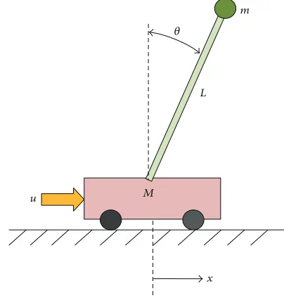
Example 9(see [31]). The last example is the fourth-order model of the inverted pendulum shown inFigure 5which is in many papers reduced to a second order system in order to verify the stability of NCSs. The pendulum mass is denoted by𝑚and the cart mass is𝑀; the length of the pendulum rod is𝐿. The open loop system is unstable. The states are defined as𝑥₁= 𝑥,𝑥₂= ̇𝑥,𝑥₃= 𝜃, and𝑥₄= ̇𝜃. The model is given by

̇

x(𝑡) =

[ [ [ [ [ [ [

0 1 0 0

0 0 −𝑚𝑔_𝑀 0

0 0 0 1

0 0 (𝑀 + 𝑚) 𝑔

𝑀𝐿 0 ] ] ] ] ] ] ]

x(𝑡) +

[ [ [ [ [ [ [ 0 1 𝑀 0 −1 𝑀𝐿 ] ] ] ] ] ] ]

𝑢 (𝑡) ,

y_{(𝑡) = [𝑥𝜃] = [}1 0 0 0_{0 0 1 0]}x(𝑡) .

(56)

The parameters used are𝑀 = 2kg,𝑚 = 0.1kg, and𝐿 =

0.5m. Then the linear model becomes

̇𝑥 (𝑡) =[[_[

[

0 1.000 0 0

20.601 0 0 0

0 0 0 1

−0.4905 0 0 0

] ] ] ]

𝑥 (𝑡) +[[_[

[ 0 −1 0 0.5 ] ] ] ]

𝑢 (𝑡) . (57)

Using the LQR Matlab function withQ = I and R = 1, the controller is given by

KLQR= [52.1238 11.5850 1.000 2.7252] . (58)

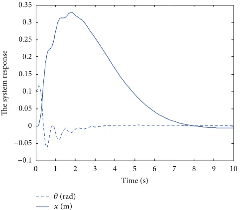
Using the LMI method the MADB is 0.0978 s and our method gives 0.0978 s usingTheorem 2andCorollary 5. We noted that there is a good agreement between our method

0 1 2 3 4 5 6 7 8 9 10

Time (s) −0.06 −0.04 −0.02 0 0.02 0.04 0.06 0.08 0.1 The syst em r esp on se

Figure 4: The response of the system inExample 7with 0.8695 s delay. u x M L 𝜃 m

Figure 5: The inverted pendulum on a cart.

and the LMI method because𝜏is small enough to make the finite difference approximation hold. The system response with 0.0978 s time delay and with 𝑥 = 0 and 𝜃 = 0.1 is shown in Figure 6 which shows the system is stable. Many examples have been studied to compare the results obtained using the method proposed in this paper with the results obtained using the LMI method [7] and the fourth-order Pade approximation method. The calculation results are summarized inTable 1along with the simulation based MADB.

Table 1: The MADB (seconds) using the proposed method with 1st, 2nd, and 3rd order finite difference approximation for the delay term, the LMI method, the fourth-order Pade approximation method, and the simulation based method.

The finite difference method

The LMI Pade approximation Simulation based

1st order 2nd order 3rd order

1 0.8695 0.8427 1.1321 0.8696 1.1672 1.180

2 0.1000 0.0995 0.1421 0.1000 0.1475 0.149

3 0.0100 0.0099 0.0149 0.0100 0.0156 0.0157

4 0.1428 0.1385 0.1808 0.1429 0.1855 0.1860

5 0.8217 0.8489 0.9085 0.8217 0.9091 0.9140

6 0.5000 0.4816 0.6303 0.5000 0.6474 0.6510

7 0.9940 0.9940 0.9960 0.9940 0.9960 0.9970

8 0.0856 0.0854 0.1192 0.0856 0.1230 0.1230

9 0.0906 0.0919 0.1251 0.0909 0.1284 0.1285

10 0.0416 0.0400 0.0496 0.0416 0.0505 0.0505

0 1 2 3 4 5 6 7 8 9 10

Time (s)

The syst

em r

es

po

n

se

−0.1 −0.05 0 0.05 0.1 0.15 0.2 0.25 0.3 0.35

𝜃(rad)

x(m)

Figure 6: The response of the system inExample 9with 0.0978 s delay.

simpler procedure, and it should have no difficulties for prac-tical design engineers to accept this approach. Clearly, the MADB with the first-order finite difference approximation is comparable with the LMI method. Furthermore, we found good agreement between the third-order finite difference approximation and the fourth-order Pade approximation. The simulation based results for the MADB show that the estimated MADB through the proposed method sufficiently achieves the system stability. A simple controller design method has been developed by the authors based on the method presented in this paper. In the controller design method a stabilizing controller can be derived for a given network time delay. In all the case studies or examples, only linear system examples are given. The method is lim-ited to linear systems only. The authors are now working on extending the methods to nonlinear systems, such as, multiconverter and inverter system and engine and electrical power generation systems [32,33].

The application of the finite difference approximation for representing the time delay is not new but we found in this paper that using higher order approximations can sufficiently represent the time delay linear system. FromTable 1 it can be concluded that using the first order approximation the estimated MADB is comparable with the other two methods. This is because the derivation of the linear model from the nonlinear model is based on neglecting the higher order derivative terms. In some cases we need to use the higher derivative terms for the time delay in order to achieve more accurate results for the MADB. The current research is to derive sufficient conditions for applying the method in order to find the tolerance of the estimated MADB.

4. Concluding Remarks

The main contribution of the paper is to have derived a new method for estimating the maximum time delay in NCSs. The most attractive feature of the new method is that it is a simple approach and easy to be applied, which can be easily interpreted to design engineers in industrial sectors. The results obtained in this method are compared with those obtained through the methods introduced in the literature. The method has demonstrated its merits in using less computation time due to its simple structure and giving less conservative results while showing good agreement with other methods. The method is limited to linear systems only and the work for extending the method for a class of nonlinear systems is on-going.

Conflict of Interests

The authors declare that there is no conflict of interests regarding the publication of this paper.

References

Mathematical Problems in Engineering 9

[2] G. C. Walsh, H. Ye, and L. Bushnell, “Stability analysis of networked control systems,” in Proceedings of the American Control Conference (ACC ’99), vol. 4, pp. 2876–2880, San Diego, Calif, USA, June 1999.

[3] G. C. Walsh, H. Ye, and L. G. Bushnell, “Stability analysis of networked control systems,”IEEE Transactions on Control Systems Technology, vol. 10, no. 3, pp. 438–446, 2002.

[4] M. S. Mahmoud,Robust Control and Filtering For Time Delay systems, Marcel Dekker, New York, NY, USA, 2000.

[5] M. S. Mahmoud and A. Ismail, “Role of delays in networked control systems,” inProceedings of the 10th IEEE International Conference on Electronics, Circuits and Systems (ICECS ’03), vol. 1, pp. 40–43, December 2003.

[6] J. E. Marshall, H. Gorecki, A. Korytowski, and K. Walton,

Time-Delay Systems: Stability and Performance Criteria with Applications, Ellis Horwood, 1992.

[7] D. Yue, Q.-L. Han, and C. Peng, “State feedback controller design of networked control systems,”IEEE Transactions on Circuits and Systems II: Express Briefs, vol. 51, no. 11, pp. 640– 644, 2004.

[8] P.-L. Liu, “Exponential stability for linear time-delay systems with delay dependence,”Journal of the Franklin Institute, vol. 340, no. 6-7, pp. 481–488, 2003.

[9] B. Tang, G. P. Liu, and W. H. Gui, “Improvement of state feedback controller design for networked control systems,”

IEEE Transactions on Circuits and Systems, vol. 55, no. 5, pp. 464–468, 2008.

[10] J. Sun, G. Liu, and J. Chen, “State feedback stabilization of networked control systems,” inProceedings of the 27th Chinese Control Conference (CCC ’08), pp. 457–461, Kunming, China, July 2008.

[11] W. Zhang, M. S. Branicky, and S. M. Phillips, “Stability of networked control systems,”IEEE Control Systems Magazine, vol. 21, no. 1, pp. 84–97, 2001.

[12] X. Li and C. E. de Souza, “Delay-dependent stability of linear time-delay systems: an LMI approach,”IEEE Transactions on Automatic Control, vol. 42, no. 8, pp. 1144–1148, 1997.

[13] W. Min and H. Yong, “Improved stabilization method for networked control systems,” inProceedings of the 26th Chinese Control Conference (CCC ’07), pp. 544–548, Hunan, China, July 2007.

[14] X.-L. Zhu and G.-H. Yang, “New results on stability analysis of networked control systems,” inProceedings of the American Control Conference, pp. 3792–3797, Seattle, Wash, USA, June 2008.

[15] M. Jun and M. G. Safonov, “Stability analysis of a system with time-delay states,” inProceeding of the American Control Conference, Chicago, Ill, USA, June 2000.

[16] K. Kim, “A delay-dependent stability criterion in time delay system,”Journal of the Korean Society for Industrial and Applied Mathematics, vol. 9, no. 2, pp. 1–11, 2005.

[17] M. S. Branicky, S. M. Phillips, and W. Zhang, “Stability of networked control systems: explicit analysis of delay,” in Pro-ceedings of the American Control Conference, pp. 2352–2357, Chicago, Ill, USA, June 2000.

[18] L. Xie, J.-M. Zhang, and S.-Q. Wang, “Stability analysis of networked control system,” inProceedings of 1st International Conference on Machine Learning and Cybernetics, pp. 757–759, Beijing, China, November 2002.

[19] A. Luis and P. J. Montestruque, “Model-based networked con-trol systems- necessary and sufficient conditions for stability,”

inProceedings of the 10th Mediterranean Conference on Control and Automation, pp. 1–58, Lisbon, Portugal, July 2002. [20] Y. Sun and N. H. El-Farra, “Quasi-decentralized model-based

networked control of process systems,”Computers & Chemical Engineering, vol. 32, no. 9, pp. 2016–2029, 2008.

[21] J. Nilsson,Real-time control systems with delays [Ph.D. thesis], Institute of Technology, Lund, Sweden, 1998.

[22] H. S. Park, Y. H. Kim, D.-S. Kim, and W. H. Kwon, “A scheduling method for network-based control systems,”IEEE Transactions on Control Systems Technology, vol. 10, no. 3, pp. 318–330, 2002. [23] Y. Zhang, Q. Zhong, and L. Wei, “Stability analysis of networked control systems with communication constraints,” in Proceed-ings of the Chinese Control and Decision Conference, pp. 335–339, July 2008.

[24] Y. Zhang, Q. Zhong, and L. Wei, “Stability analysis of networked control systems with transmission delays,” in Proceedings of the Chinese Control and Decision Conference, pp. 340–343, July 2008.

[25] J. Wang, ¨U. Kotta, and J. Ke, “Tracking control of nonlinear pneumatic actuator systems using static state feedback lin-earisation of input/output map,” Proceedings of the Estonian Academy of Sciences: Physics, Mathematics, vol. 56, no. 1, pp. 47– 66, 2007.

[26] D. P. Goodall and J. Wang, “Stabilization of a class of uncertain nonlinear affine systems subject to control constraints,” Interna-tional Journal of Robust and Nonlinear Control, vol. 11, no. 9, pp. 797–818, 2001.

[27] J. Wang, J. Pu, P. R. Moore, and Z. Zhang, “Modelling study and servo-control of air motor systems,”International Journal of Control, vol. 71, no. 3, pp. 459–476, 1998.

[28] C. D. Meyer,Matrix Analysis and Applied Linear Algebra, SIAM, 2000.

[29] F. Yang and H. Fang, “Control strategy design of networked control systems based on maximum allowable delay bounds,” inProceedings of the IEEE International Conference on Control and Automation (ICCA ’07), pp. 794–797, Guangzhou, China, June 2007.

[30] P. Naghshtabrizi, Delay impulsive systems: a framework for modeling networked control systems [Ph.D. thesis], University of California, Los Angeles, Calif, USA, 2007.

[31] K. Ogata,Modern Control Engineering, Prentice Hall, New York, NY, USA, 3rd edition, 1997.

[32] J. L. Wei, J. Wang, and Q. H. Wu, “Development of a multi-segment coal mill model using an evolutionary computation technique,”IEEE Transactions on Energy Conversion, vol. 22, no. 3, pp. 718–727, 2007.

Submit your manuscripts at

http://www.hindawi.com

Hindawi Publishing Corporation

http://www.hindawi.com Volume 2014

Mathematics

Hindawi Publishing Corporation

http://www.hindawi.com Volume 2014 Mathematical Problems in Engineering

Hindawi Publishing Corporation http://www.hindawi.com

Differential Equations

International Journal of

Volume 2014

Hindawi Publishing Corporation

http://www.hindawi.com Volume 2014 Hindawi Publishing Corporationhttp://www.hindawi.com Volume 2014

Hindawi Publishing Corporation

http://www.hindawi.com Volume 2014

Mathematical PhysicsAdvances in

Complex Analysis

http://www.hindawi.com Volume 2014

Optimization

Hindawi Publishing Corporation

http://www.hindawi.com Volume 2014

Combinatorics

Hindawi Publishing Corporation

http://www.hindawi.com Volume 2014 International Journal of

Hindawi Publishing Corporation

http://www.hindawi.com Volume 2014

Journal of

Hindawi Publishing Corporation

http://www.hindawi.com Volume 2014

Function Spaces

Abstract and Applied Analysis

Hindawi Publishing Corporation

http://www.hindawi.com Volume 2014

International Journal of Mathematics and Mathematical Sciences

Hindawi Publishing Corporation http://www.hindawi.com Volume 2014

The Scientific

World Journal

Hindawi Publishing Corporation

http://www.hindawi.com Volume 2014

Hindawi Publishing Corporation

http://www.hindawi.com Volume 2014

Discrete Dynamics in Nature and Society

Hindawi Publishing Corporation

http://www.hindawi.com Volume 2014

Hindawi Publishing Corporation

http://www.hindawi.com Volume 2014

Discrete Mathematics

Hindawi Publishing Corporation

http://www.hindawi.com Volume 2014 Hindawi Publishing Corporationhttp://www.hindawi.com Volume 2014