Improving the Convergence Rate of
Rotorcraft Loose Coupling Algorithms
using Interaction Laws based on
Autoregressive Modelling
Master’s Thesis
Maarten Bosmans
University of Twente — National Aerospace Laboratory NLR
Abstract
Problem area
In many dynamical systems, the physics of the overall system can be modelled as the interaction between several subsystems, each governed by its own laws of physics. A prime example of this is rotorcraft flight, where aerodynamics and structural mechanics are closely coupled. In order to simulate the dynamics of rotorcraft flight, a widely used approach is a Loose Coupling, in which a structural dynamics model and a (computationally expensive) fluid dynamics model are combined with a simplified aerodynamics model. However, even with a loose coupling approach the fluid dynamics model needs to be solved many times before a coupled solution is found. The goal of the present work is to reduce the amount of computational work needed for accurate rotorcraft aeroelastic simulation.
Description of work
A one-dimensional model problem is constructed that resembles the rotorcraft simulation in a very simple way. It is expected that established techniques from time series analysis can be used to improve the convergence of the coupled models. Using the model problem various methods for improving the loose coupling are evaluated.
Results and conclusions
The time series resulting from the convergence of the loosely coupled procedure can accurately be modelled as an autoregressive process. This model is subsequently used to estimate the final solution of the iterative procedure, improving the overall convergence rate.
Applicability
Contents
1 Introduction 5
2 Interaction laws 7
2.1 General formulation 7
2.1.1 Introducing the interaction law
2.2 Fluid–structure interaction with heat transfer 10
2.3 Viscous boundary layer interaction 11
2.3.1 The iterative procedure and interaction law 2.3.2 Analysis of the interaction law
2.4 Loose coupling in rotorcraft fluid–structure interaction 14 2.4.1 Loose coupling as an interaction law
2.4.2 Remarks on the loose coupling approach
3 Autoregressive modelling of time series 19
3.1 Autoregressive model 19
3.1.1 Parameter estimation
3.2 Vector Autoregressive model 20
3.2.1 Subset VAR model
4 Model problem 23
4.1 Governing Equations 23
4.1.1 Boundary conditions and model coupling 4.1.2 Nondimensionalisation
4.2 Fluid discretisation 25
4.2.1 Numerical flux 4.2.2 Boundary conditions 4.2.3 Iterative solution strategy
4.3 Structure discretisation 30
4.4 Coupling methods 30
4.4.1 Tight coupling 4.4.2 Loose coupling
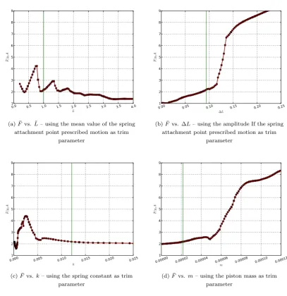
4.5 Trim adjustment 33
4.5.1 Choosing a trim parameter 4.5.2 Effect of trim on the simple model 4.5.3 Trim solution strategy
5 Evaluation of the model problem and coupling strategies 39
5.1 Untrimmed FSI coupling 39
5.1.1 Convergence to a periodic solution 5.1.2 Comparison with the simple model
5.2 Coupled model with trimming 43
5.2.1 Tight coupling 5.2.2 Loose coupling
6 Improving the loose coupling convergence 49
6.1 Relaxation 49
6.1.1 Relaxation on∆p
6.1.2 Relaxation onz
6.1.3 Disadvantages of relaxation with a fixed parameter 6.1.4 Aitken relaxation
6.1.5 Summary of results for relaxation
6.2 A basic autoregressive model 55
6.2.1 An alternative expression for the convergence criterion 6.2.2 Estimation of ∆p
6.2.3 Adjustment of∆p
6.2.4 Application of the adjustment 6.2.5 Summary of the results
6.3 Improving the AR model 60
6.3.1 Using more of the history ofPn
6.3.2 Using the whole vector∆p
6.3.3 Using a higher order AR(p) model 6.3.4 A simple VAR approach
6.3.5 A subset VAR approach using only diagonal entries 6.3.6 A VAR approach using the average as reference 6.3.7 Including more nonzero elements
6.3.8 An AIC-based subset VAR approach
6.4 Comparison of autoregressive techniques 68
7 Conclusions 71
Acknowledgements 75
Bibliography 76
A List of variables and parameters 78
CHAPTER
1
Introduction
Rotorcraft aerodynamics is considerably more complex than that of fixed wing aircraft. The high aspect ratio and flexibility of the rotor blades result in a complex interplay between the inertial and elastic forces in the structure and the aerodynamic forces acting on the blades. Depending on flight conditions, the wake of the rotor can interact with the fuselage, tail rotor or the rotor itself. An important and characteristic example of such an interaction is known as blade–vortex interaction (BVI). Vortices coming off a rotor blade tip remain in the path of the rotor and interact with one of the next blades. This can be the cause of large force fluctuations on the rotor blade. The resulting blade deformations are the cause of the typical, loud sound produced by a helicopter rotor.
To simulate rotorcraft flight, both computational structural dynamics (CSD) and computa-tional fluid dynamics (CFD) play an important role. An accurate mathematical model of the structure is needed to calculate the blade deformation under load. The CFD model needs to cap-ture aerodynamic properties not only accurately, but also efficiently. The most straightforward way to solve the coupled structural and fluid equations is to combine them into a single formu-lation. This is called a monolithic scheme. In practice, however, especially in applied rotorcraft research, a monolithic approach is almost never used, because it is difficult to integrate the two different systems of equations in a single numerical procedure. More common are partitioned schemes in which separate CSD and CFD solvers are used to solve the combined system. This ap-proach has advantages in computational efficiency and software modularity, for example because the models and implementations can follow the state of the art in each field separately. Only a monolithic scheme can, however, maintain the conservation properties of the mathematical mod-els it is based on at the CSD-CFD interface. Conservation requires strict compatibility on the approximation spaces at the interface and other conditions on the discretisation, see [1], [2]. A partitioned scheme can, however, be modified to be higher order accurate in energy conservation ([3]).
done in a staggered approach, where the models are evaluated at interleaved points in time. Loose coupling removes the requirement of information exchange at each time step. The models are time-integrated separately and are only coupled e.g. once every rotor revolution. The structural model calculates the blade motion for an entire revolution using a simplified model of the aerodynamic forces on the rotor blades. This approximation can come from lifting line theory or from an experimentally found lookup table. The coupling is then achieved by transferring the calculated blade motion to the CFD model and using the computed airflow solution to find better blade loads.
The advantages of a loosely coupled scheme become apparent if one takes rotor trim into account. Because directly comparing experimentally measured trim angles with the simulated results often leads to large discrepancies, the usual approach is to prescribe the total loads on the rotor hub and let the simulation solve for trim. This procedure adds another level of iteration for the convergence of the trimmed coupled system. For tight coupling this results in a procedure that is currently [4] deemed too expensive. With loose coupling, however, the rotor trim can be adjusted during the rotor structural calculations using the simplified aerodynamics model. This is especially useful in the case of steady flight conditions, when the solution is assumed to be periodic.
In the field of financial and statistical modelling a lot of problems are presented as a time series. A time series is a set of data points corresponding to observations of a particular process at different times. In econometrics a time series can for example be the price of a stock at the start of the trading day. Another example application of time series analysis comes from climate research, where the atmospheric history can be studied using the width of tree rings as the time series.
The goal of time series analysis is to extract some properties from the time series that char-acterise the underlying process. A large and important class of models that is used to describe time series is that of the autoregressive models. These models correlate the current data point with a finite or infinite number of previous points of the series with a linear system of equations. When the model is fitted to all the past observations of the time series, it can be used to predict the future course of the series.
The goal of the present work is to analyse and improve the loose coupling of an aeroelastic rotor simulation for trimmed periodic flight conditions.
The loose coupling of the three models (CFD, CSD and trim) will be formulated as an in-teraction law, in order to compare it to other uses of inin-teraction laws in the literature. A one-dimensional model problem is constructed that resembles the rotorcraft simulation, includ-ing the trimminclud-ing process, in a very simple way. Usinclud-ing the model problem several methods for improving the loose coupling are proposed. It is expected that established techniques from time series analysis can be used to improve the convergence of the coupled models.
CHAPTER
2
Interaction laws
Using a partitioned scheme to solve problems involving complex interaction can be challenging with respect to stability and convergence. A possible approach to overcome these problems is the use of an interaction law. An interaction law replaces the boundary condition on the partition boundary in one model with an alternative boundary condition. The new boundary condition approximates the physics of the other model, without actually using the other model. This way the models of which the partitioned scheme is composed of are decoupled. Usually this interaction law is chosen as simple as possible, while retaining enough characteristics of the original model to enhance convergence of the coupled system.
In this chapter the role of the interaction law on a coupled system will be investigated. First some notation will be introduced so that the different interaction laws can be described in a similar manner. Then two examples from the literature are presented in which interaction laws play a role in the convergence behaviour of a coupled system. The second example, in Section 2.3, also includes some analysis about how the interaction law influences the coupled system. Finally, in the last section the concept and notation of an interaction law are applied to the loose coupling approach for rotorcraft aeroelastic modelling.
2.1. General formulation
To formalise the concept of an interaction law in the context of coupled systems, a general formulation is given. LetS andF be the structural and fluid model with internal statexandy respectively. The two models are coupled by requiring that some set of variables defined for both models have unique values on the interaction surface Γ. These variables do not necessarily have to be part of the internal state, but should be readily computable from it, using the functions
SΓ:Rnx 7→
RnΓ andFΓ: Rny 7→
RnΓ. The combined system can be described as
S(x) = 0
F(y) = 0
SΓ(x) =FΓ(y).
(2.1)
Instead of finding a solution for this system using a direct method, an iterative method is used. In an iterative procedure the models are alternatingly solved until both are converged to a fixed point. Instead of prescribing all the variables on Γ for both models, the set of variables is partitioned into two parts. For one of the parts the values of the variables fromFΓ are used
forFΓ.
SΓ(x) =
"
Sl
Γ(x) Sr
Γ(x)
#
FΓ(y) =
"
Fr
Γ(y) Fl
Γ(y)
#
with
Sl
Γ(x),F
r
Γ(y)∈R
n1
Sr
Γ(x),FΓl(y)∈Rn2
n1+n2=nΓ
The parts are called the left and right part, according to the side on which they appear in the iterative procedure. The iterative procedure is given by
(
S(xn) = 0
SΓl(x
n
) =FΓr(y
n−1)
(
F(yn) = 0
Fl
Γ(y
n) =Sr
Γ(x
n).
(2.2)
In this general formulation it is not important how the modelsS andF are solved. In practice an iterative method could very well be used for each of the models, resulting in a nested iterative approach.
In the context of a helicopter rotor aeroelastic simulation, S could be the CSD model of the rotor blade withxthe deflection angles along the blade axis. F is the CFD model withy the flow state, for example the density, fluid velocity and specific energy for all the grid points. A possible way of coupling the systems is to letFr
Γ(y) be the aerodynamic pressure of the airflow
on the rotor blade andSr
Γ(x) the position and velocity of the blade. Every iteration of S then
solves the blade deflections using the aerodynamic forces and subsequentlyF solves the airflow around the blade with the blade motion prescribed as a boundary condition.
It is important to note that if (2.2) converges, it will converge to a solution of (2.1). For if yn =yn−1 thenSl
Γ(x
n) =Fr
Γ(y
n) andSr
Γ(x
n) =Fl
Γ(y
n). By construction then alsoSΓ(xn) =
FΓ(yn).
2.1.1. Introducing the interaction law
An interaction law emerges from the observation that if Sl
Γ(x
n) could be solved with Fr
Γ(y
n)
instead ofFr
Γ(y
n−1), the procedure would converge in one step. However, solvingFr
Γ(y
n) together
withSl
Γ(xn) reduces the iterative procedure to a direct method again, negating the advantage in
computational complexity of the iterative method. So instead an approximation ˜Fr
Γ is used that
approximates the behaviour of Fr
Γ(yn) using only yn−1 (and possibly xn). The new coupling
equation resulting from the use of the approximation is called the interaction law. A possible interaction law could be based on a linearisation of Fr
Γ aroundyn−1 Fr
Γ(y
n)≈ Fr
Γ(y
n−1) + ∂FΓr
∂y yn−1
yn−yn−1. (2.3)
This formulation still containsyn, so it is not suitable yet to be used in (2.2). Linearisation of
Fl
Γ aroundy
n−1and applying the result toyn yields
FΓl(y
n) =
FΓl(y
n−1) + ∂FΓl
∂y yn−1
(yn−yn−1).
This equation can be rewritten using the relationFl
Γ(yn) =SΓr(xn) to Sr
Γ(x
n)− Sr
Γ(x
n−1) = ∂FΓl
∂y yn−1
(yn−yn−1).
Using this equation in (2.3) requires inverting the Jacobian ofFl
Γ and yields Fr
Γ(y
n)≈ Fr
Γ(y
n−1) +
" ∂Fr
Γ
∂y ∂Fl
Γ
∂y −1#
yn−1
Sr
Γ(x
n)− Sr
Γ(x
n−1)
. (2.4)
This approximation of Fr
Γ(y
n) could already be used to replace Fr
Γ(y
n−1) in (2.2), because it
only depends on known variables (yn−1 andxn−1) and on the state of the model that is to be
solved (xn). To simplify the calculation of the interaction law, a simple model is introduced.
Using a simple model
The Jacobian matrices in (2.4) can be very large, because they both involvey, the complete internal state of F. Furthermore the second Jacobian is generally not invertible, because the stateycontains much more elements than the boundary conditions forF. However, the product of the Jacobian and the inverse Jacobian is a much smaller matrix. The idea of the interaction law is that this smaller matrix does not need to be computed directly, but can be replaced by a similar matrix and the advantages of better convergence still hold.
This is where the simple model is introduced, as an approximation of the combined Jacobians. As said, the simple model need not be the exact solution of the combined Jacobians, but can be anything with the same general behaviour. Often it is derived from some sort of physical interpretation, using a very simple representation, which can be easily (in a direct way) calcu-lated. This simple model ˜F thus can be seen as a map from the boundary condition ofF to the boundary condition ofS. The complete interaction law to be used as a replacement for Fr
Γ in
(2.2) is now
˜
Fr
Γ=F
r
Γ(y
n−1) + ˜F Sr
Γ(x
n)− Sr
Γ(x
n−1)
. (2.5)
When this interaction law is used in (2.2) instead of Fr
Γ the boundary condition for S is
changed. In the case that ˜F is linear the new boundary condition can be written with all the unknown terms on the left hand side.
Sl
Γ(xn)−F˜(SΓr(xn)) =FΓr(yn−1)−F S˜ Γr(xn−1)
The boundary condition is now more complex, with an extra term containingxnon the left hand
side of the equation. IfS itself is solved using an iterative procedure this means that the simple model ˜Fhas to be calculated many times. So eachS–F iteration becomes more computationally expensive. But as the simple model should have the same general behaviour asF, it is expected that there are lessS–F outer iterations necessary.
A desirable property of an interaction law is that although it may change the convergence path, the solution of the converged system is the same as the solution of the original coupled system. For the interaction law as formulated in (2.5) this property holds if ˜F is linear and Sr
Γ is continuous. It can be seen that this is the case by noting that when xn → x¯ then also
SΓr(xn)→SΓr(¯x) under continuity ofSΓr. The contribution of ˜F in (2.5) then vanishes due to its linearity. So if the new procedure converges, the approximated ˜Fr
Γis exactly equal to the original Fr
Γand the new procedure converges to the solution of the original partitioned system, regardless
of the choice for ˜F. Of course the choice of the simple model does influence the convergence of the iterative procedure. If the simple model does not reflect the behaviour of the original model
The interaction law detailed above is only a example. A variation of this interaction law that will be used later is
˜
Fr
Γ =FΓr(yn−1) + ˜F(SΓr(xn))−F S˜ Γr(xn−1)
. (2.6)
This interaction law loosens the requirement on ˜F and only requires it to be continuous.
2.2. Fluid–structure interaction with heat transfer
Interaction laws can be used in all sorts of problems involving partitioned procedures. For exam-ple in [5] passenger comfort in an aircraft cabin is modelled. This is done by coupling a human body thermoregulation model, an airflow model and a radiation model. The thermoregulation modelT and the flow modelFare coupled by the requirement that the temperatureT and heat flowqon the body surface are the same for both models. The models and their coupling can be described as
T(x) = 0
F(y) = 0
TΓ(x) =FΓ(y)
(2.7)
withTΓ(x) = "
qb
Tb
#
, FΓ(y) = "
qf
Tf
# .
The vectorsT andqare of equal length and the modelsT andF are well-posed if exactly one of these vectors is prescribed. The coupled system can be solved with an iterative procedure by specifyingqb=qf as a boundary condition forT andTf =Tb forF.
Tl
Γ(x
n) =qn
b F
r
Γ(y
n−1) =qn−1
f
Fl
Γ(y
n) =Tn
f T
r
Γ(x
n) =Tn b
Of course the role of temperature and heat flux could also be reversed. Both these approaches were tried in [5], but it was found that neither resulted in a stable procedure.
The seemingly arbitrary distinction between the temperature as a boundary condition for one model and the heat flow for the other suggests that it might be fruitful to use an approach which is symmetric with respect to the variables used in the coupling. To this end an interaction law is introduced for both the models. The interaction laws use a simple model to characterise the other system. Each simple model is based on a linearisation using a heat-transfer coefficienth to characterise the system it represents.
qb =hb(T0−Tb) qf =hf(Tf−T∞),
(2.8)
withT0andT∞suitable reference temperatures in the body and airflow respectively. Now instead
of usingTl
Γ(x
n) =qn−1
f as the boundary condition for T, (2.8) is used to find the estimate ˜q n f
using some fixedhf. As the heat-transfer coefficienthf is not known yet for the current iteration, hnf−1 is used as an approximation. Also Tfn is not known yet, but from boundary condition for
Fl
Γ it can be seen that it must be equal toT
n
b. This leads to the revised boundary condition
˜
Fr
Γ= ˜q
n f
=hf(Tfn−T∞)
=hnf−1(Tbn−T∞).
Similarly, the flow model is solved using the new boundary condition ˜
Tr
Γ =T0−
qn f hn b .
Using (2.8) to eliminate hn−1 from these equations, the revised boundary conditions of the interaction law emerge
˜
Fr
Γ =q
n−1
f
Tbn−T∞
Tfn−1−T∞
˜
Tr
Γ =T0+
qnf
qn b
(Tbn−T0).
In [5] the original system (2.7) is solved using these revised boundary conditions. The inter-action law stabilises the system and the iterative procedure now converges.
To see why the coupling between the two models is now symmetric, the coupling equations can be rewritten. From the form in which they appear in the original paper,
qbn= (Tbn−T∞)hnf−1 qfn= (T0−Tfn)h
n b,
it is clear that with the application of the interaction law the arbitrary distinction between the prescribed variables on the model boundaries is removed. The physical interpretation of this is that the Dirichlet and Neumann boundary conditions in the original system are replaced by a mixed boundary condition for both models.
2.3. Viscous boundary layer interaction
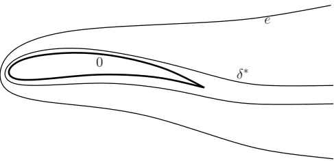
Another example of an interaction law involves the viscous–inviscid interaction described by Veldman in [6] and [7]. In an attempt to reduce the computational effort of simulating viscous airflow around an airfoil, viscous flow is only calculated in a small layer around the airfoil. In the flow domain outside the viscous layer, the airflow is assumed to be inviscid. The models are coupled by requiring the density and flow speed of both models to be the same on the interface between the viscous and inviscid flow,e.
In the viscous region the boundary-layer equations are used, which describe a thin boundary layer around the airfoil. The influence of the boundary layer on the inviscid airflow is modelled by a displacement effect, i.e. the airfoil appears thicker due to viscous effects. This displacement δ∗ of the airfoil is incorporated in the inviscid model by using a surface transpiration concept, where a non-zero normal velocity on the original airfoil boundary is prescribed. The boundary condition for the inviscid model is
ρ0v0=
∂ ∂x(ρeueδ
e
δ∗
[image:14.595.164.408.80.198.2]0
Figure 2.1.:Viscous–Inviscid interfaceeand displacement thicknessδ∗, both exaggerated in thickness
withρ0v0 the mass flux normal to the airfoil andρeuethe stream-wise mass flux at the edge of
the viscous layer.
For the purpose of this research the exact equations used to describe the viscous and inviscid physics of the airflow are not important. It suffices to say that for a given airfoil geometry and upstream flow conditions, both models can be expressed as a relation between the coupled variables,ue andδ∗.
2.3.1. The iterative procedure and interaction law
In the work of Veldman the viscous model and the external inviscid flow are defined asue=V(δ∗)
andue=E(δ∗). Here the notation of Equation (2.2) will be used, in order to see the connection
with the general formulation of an interaction law. A straightforward iterative procedure could be written as
V(xn) = 0
VΓl(x
n) =
EΓr(y
n−1) =un−1
e
E(yn) = 0
El
Γ(y
n) =Vr
Γ(x
n) =δ∗n.
(2.9)
Here V(x) =ue−V(δ∗) and E(x) =ue−E(δ∗). The internal states xand y both contain ue
andδ∗ along the airfoil, in some not further specified way.
This procedure produces correct results for attached flows, but according to [6] it breaks down when flow separation occurs. Near the singular points of flow separation there is a strong interaction between the viscous and inviscid flow and no hierarchy between the models is present. The viscous model used forVhas a minimum forue, corresponding to the onset of flow separation.
The iterative procedure breaks down whenuebelow this minimum is prescribed forV. Reversing
the order of information exchange solves this problem, asV can be solved for anyδ∗, but leads to a very slow converging procedure.
An interaction law is used to obtain a stable procedure, while still solving the original combined system with as little extra computational work as possible. The interaction law consists of a simple model as an approximation of E. This simple model is solved simultaneously with the boundary-layer equations ofV. The effect of this is that the boundary condition forV is not just ue anymore, but also contains the simple model. This results in a stable procedure, even in the
presence of flow separation.
Usually the simple model is based on some physical representation that is simpler than that ofE. But this can lead to interaction laws that are still quite complex and increase the
putational work required to solveV together with the simple model substantially. Because the interaction law does not influence the solution resulting from the iterative procedure, it is not strictly necessary that the simple model is derived from a physical representation of the system it describes. In order to keep the interaction law simple, the proposed simple modelI:ue=I(δ∗)
is constructed in a straightforward way based on the matrices describing the numerical models. Let V, E and I be the matrix representation of the V, E and I respectively. In the no-tation of Equation (2.9), V and E are the matrix representation of [0|Id]T
V|Vl
Γ
(Vr
Γ) −1
and
Er
Γ
E|El
Γ
−1
[0|Id], with Idthe identity matrix and|the matrix stacking operator.
The simple model is constructed by dropping off-diagonals ofE. This means thatIcan vary from very simple, a matrix containing only the main diagonal ofE, to a complete copy of E. The proposed revised iterative procedure as formulated in the original paper is
(I−V)δ∗n= (I−E)δ∗n−1. (2.10) Formulated as an interaction law the similarity to (2.6) is clear.
˜
Er
Γ=une−1+ I(δ∗n)− I(δ∗n−1)
In [7] it is shown that this interaction law results in a procedure that can solve the coupled system in the presence of flow separation, except for the degenerate case I = E, i.e. no off-diagonals are dropped. Even when I is reduced to the least possible complexity, a diagonal matrix, the interaction law results in a stable procedure and the coupled system converges.
2.3.2. Analysis of the interaction law
To see why the interaction law results in a stable procedure, some matrix theory is required. Statements here are based on theorems developed in [8] and [9]. Exact references and more details can be found in [6] and [7].
First, E−V and I−V are assumed to be diagonally dominant and have positive diagonal entries and non-positive off-diagonals, with all the eigenvalues in the stable half-plane. These conditions onE−Vlead to the fact thatE−Vis non-singular and (E−V)−1≥0. The iterative procedure (2.10) is the repeated application of the operator (I−V)−1(I−E). The maximum
absolute value of the eigenvalues, the spectral radiusρ, of this operator is strictly less than unity. ρ (I−V)−1(I−E)<1
This means that the iterative procedure (2.10) is convergent and that it converges to (E−V)δ∗= 0.
Moreover, if two matrices Ia and Ib are both simplifications of E, where Ib has more off-diagonals dropped or thanIa, that isIa≤Ib, then the spectral radius of the iterative operator ofIais not greater than that ofIb.
ρ (Ia−V)−1(Ia−E)
≤ρ (Ib−V)−1(Ib−E)
.
This means that the number of iterations required to solve (2.10) increases monotonically with the number of off-diagonals dropped fromE.
number of these sub-iterations decrease monotonically in the number of dropped off-diagonals in
I.
The two iterative processes show opposite convergence behaviour when the interaction law
I is simplified. To find the method with the overall lowest number of iterations, numerical experiments have been performed by Veldman. In [7] it is shown that for both the simplest interaction law, where only the main diagonal remains, and for the caseI→E, the total number of sub-iterations required reaches a local minimum.
For the original problem to converge to a solution, all eigenvalues ofE−V should lie in the stable half-plane. As a measure of robustness, let τ( . ) denote the minimum real part of the eigenvalues of a matrix. Then under the earlier assumptions forE−VandI−Vit can be shown that
τ(E−V)≤τ(Ia−V)≤τ(Ib−V),
withIa≤Ib. So robustness of the interaction law increases as more off-diagonals are dropped. An outline of the proof follows. By construction we have
E−V≤Ia−V≤Ib−V.
Now if each of these these three matrices are decomposed asA=αId−Aˆ, withαsufficiently large such thatAˆ ≥0, then the Perron–Frobenius theorem can be used. This theorem states that ifAˆ ≥0 is an irreducible matrix then Aˆ has a positive real eigenvalue equal to its spectral radiusρ(Aˆ) andρ(Aˆ) increases when any entry ofAˆ increases.[9]
So if ˆλis the largest real eigenvalue ofAˆ, thenτ(A) =α−λˆ. Moreoverτ(A) is non-decreasing inA, which concludes the proof.
2.4. Loose coupling in rotorcraft fluid–structure interaction
Current research on the simulation of steady forward rotorcraft flight is generally based on a loose coupling method between a rotorcraft flight dynamics model and an aerodynamics solver using, for example, the Euler [10] or Reynolds-averaged Navier–Stokes [11] equations. The flight dynamics model usually consists of a CSD model describing the structure of the rotor blades, integrated with a simplified CFD model for the aerodynamics and a trim procedure. The sim-plified aerodynamics model can be a lookup table of experimentally found aerodynamic forces or a lifting line model, possibly extended by including unsteady effects and a vortex wake. The simplified model is usually called the 2D-CFD model, as it does not compute a full 3-dimensional flow solution. The trim procedure adjusts the angles of the flight controls, which prescribe the motion of the rotor blade at the root. The goal of the trim procedure is to adjust the control angles such that the resulting mean total rotor hub loads are appropriate for the chosen flight condition.
In order to make the results of the flight dynamics model more accurate, it is coupled to a first principles CFD model. The loose coupling procedure is outlined below and also shown in Figure 2.2.
• The flight dynamics code computes a trimmed periodic solution of a full rotor revolution. This results in blade deformationxand aerodynamic forces (calculated by the simplified model) on the rotor bladeF2D.
• The CFD grid is deformed according toxand a flow solution is calculated. This results in more accurate aerodynamic forcesF3D.
• The difference between the two aerodynamic loads is calculated, ∆F =F3D−F2D. This delta load can be seen as the error of using the 2D model in the calculation of the flight dynamics.
• The rotor is trimmed again by the flight dynamics model. The total aerodynamic loads used in the trimming process is the sum of the forces calculated by the simplified model and ∆F from the last CFD solution.
• The previous three steps are repeated until convergence is achieved.
The system is said to be converged if the total loads and pitch angles do not significantly change from one coupling iteration to the next. In general if the 2D-CFD model is good enough, the loose coupling will converge without the need for relaxation.
CSD
Trim
aerodynamic loads
blade deformation
total hub loads
pitch angles
CFD
CFD
2Ddelta loads
blade deformation
Flight Dynamics
Figure 2.2.:Schematic overview of the loose coupling approach
2.4.1. Loose coupling as an interaction law
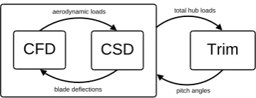
To see how this loose coupling approach fits in the framework laid out in Section 2.1, the proce-dure described above is presented in the formulation of Equation (2.2). First the three models and their relations are stated on a conceptual level. Then an iterative procedure for solving this combined system is proposed and finally it is shown that applying an interaction law permits the resulting procedure to be transformed into the loose coupling approach.
The basic coupled system, without using a 2D-CFD model, consists of three parts: a CSD and CFD model and a trim procedure. These three parts and their relations can be described as
S(x) = 0
F(y) = 0
T(L, θ) = 0
SΓ1(x) =FΓ1(y)
SΓ2(x) =TΓ2(L, θ).
(2.11)
HereS andF are the CSD and (full) CFD models, with the blade deflectionsxand fluid flow statey. T is the trim procedure. For clarity its variablesL, the mean total rotor hub loads, and θ, the control angles, are written separately. It is important to note thatxandy represent the blade deformation and flow state for every time step in an entire rotor revolution of the periodic solution. The combined system is to be solved for the free variableθwith prescribedL.
CFD
CSD
Trim
aerodynamic loads
blade deflections
total hub loads
[image:18.595.196.376.81.150.2]pitch angles
Figure 2.3.:Schematic overview of a basic iterative approach
superscriptnfor the iterations in the inner loop and superscriptk for the outer iterations, the iterative procedure is
S(xn) = 0
SΓl1(x
n) =F3D(yn−1) Sl
Γ2(x
n) =θk−1
(
F(yn) = 0
Fl
Γ1(y
n) =xn
(
T(Lk, θk) = 0
Tl
Γ2(L
k, θk) =L(xk).
(2.12)
First, the CSD and CFD models are iteratively solved with a fixed trim angleθk−1. The boundary condition ofS consists of the aerodynamic forcesF3Dand the boundary condition ofF are the
blade deflectionsx. When this combined procedure has converged the solution of the CSD model xk is used to calculate the mean rotor hub loadsL. Using the difference between thisLand the
target loads, the trim procedureT calculates the newθk and the next outer iteration can begin.
In order for the trim procedure to be able to calculateθk, it must have some knowledge of the
effect of adjustments toθ onL. This can be for example an (estimated) influence matrix ∂L∂θ.
Adding the simplified aerodynamics
In order to speed up the convergence of the coupled system, an interaction law is introduced. The interaction law used instead ofF3D is very similar to the one shown in Equation (2.6). S
will be solved with ˜F3D, an approximation forF3D(yn), instead ofF3D(yn−1). In the interaction
lawF2D, the aerodynamic forces on the rotor blade as calculated by the simplified model, is used to estimate the difference betweenF3D(yn−1) andF3D(yn).
˜
F3D=F3D(yn−1) + F2D(xn)−F2D(xn−1)
The goal of the interaction law is to allow the combined system to be solved with fewer iterations of the (computationally intensive) CFD model. This is done by moving theF from the inner to the outer loop. To make that possible, first the terms of ˜F3D are reordered, such
that a delta load as used in the loose coupling procedure appears. ˜
F3D=F2D(xn) + F3D(yn−1)−F2D(xn−1) =F2D(xn) + ∆Fn−1
Now instead of updating ∆Fn in every iteration ofS, a fixed ∆F is used. The result of this is that the CSD and CFD models are detached. The boundary condition ˜F3Dand thus the solution
procedure forS does not depend anymore on information fromF at inner iterationn−1. This
allows forF and T to swap places in the iterative procedure, such that the S–T iterations are now the inner loop and the (ST)–Fiterations are the outer loop. The revised iterative procedure using the interaction law is then described by
S(xn) = 0
SΓl1(x
n) =F2D(xn) + ∆Fk−1 SΓl2(x
n) =θn−1
(
T(Ln, θn) = 0
Tl
Γ2(L
n, θn) =L(xn)
(
F(yk) = 0
Fl
Γ1(y
k) =xk
with ∆Fk=F3D(yk)−F2D(xk).
(2.13)
This procedure to solve the original system (2.11) is exactly the formalised version of the described loose coupling approach.
2.4.2. Remarks on the loose coupling approach
The role of the interaction law
It is important to note that the primary goal of the interaction law for the loose coupling approach is different than for the examples described in Section 2.2 and 2.3. These previous examples involved only two coupled models and the interaction law was necessary to facilitate convergence of the coupling iterations. In contrast, the case described here involves three models that have to be coupled. Also, in general the stability of the S–F coupling is not a problem for practical rotorcraft aeroelastic simulations. The main problem is the computational load required for solving the CFD model to the required accuracy without a prescribed trim.
While the interaction law will also have a positive influence on the convergence of the coupled system, its main purpose here is to enable the CFD model to be moved to the outer loop. This reduces the number of times this computationally expensive model needs to be solved.
Hierarchy in model coupling
The iterative treatment of the three coupled models has been shown with two different hierarchies. The first withS–F in the inner loop and the second withS–T in the inner and F in the outer loop. This suggests the possibility of a third method, in which the inner loop consists ofF–T
and the CSD model is solved in the outer loop.
Because F andT are not directly coupled, but only indirectly throughS, there is nothing to iterate in the inner F–T loop. Thus this approach is actually the same as a non-hierarchical approach, in which the three models are solved consecutively in one iterative loop. The indepen-dence ofF and T in the inner loop could be exploited by solving the two models at the same time, in parallel. However for rotorcraft simulation this has no practical advantages, because solvingT is trivial compared to solvingF.
The model hierarchy with anS–Finner loop could also be restored using an approximation of
approachF still resides in the inner loop of the hierarchy, with the corresponding computational disadvantages, as discussed earlier.
Convergence and consistency of the modified procedure
Provided that the problem of solving the combined model is well posed, the choice of model for the simplified aerodynamics does not influence the solution of the converged system. For if the loose coupling converges thenxn =xn−1 and thus F2D(xn) =F2D(xn−1). So in the boundary
conditionSl
Γ1 from (2.13) the twoF
2D terms cancel and onlyF3D(yk−1) remains. This means
that the loose coupling as described by (2.13) will converge to the same solution as the original procedure (2.12), irrespective of the choice of the simple modelF2D. Of course it is still possible
that the loose coupling is not stable at all, perhaps even when the original procedure is. In particular, it is expected that when the simple model is not a sufficiently good approximation of the CFD model, the loose coupling will fail to converge.
In [10] it was shown that for a practical rotorcraft aeroelastic coupling the choice of 2D model did have an influence on the solution of the coupled system. The solution was different when another simplified model was used and neither matched the tight coupling solution used as a reference. This was attributed to the fact that the CSD and CFD models were only coupled in a few variables along the rotor blade. If for example only lift and drag are coupled between the CFD model and the structural model and the lifting line 2D model additionally calculates a pitching moment, the solution will depend on the choice of 2D model.
Another possible reason for different solutions found by the loose coupling is that the problem of finding a trimmed solution is not well posed at all, i.e. there are multiple solutions. As the choice of interaction law does influence the convergence path, it is possible that by changing the 2D model a different solution is found. This does not have to be a problem however, because both solutions are equally valid. The solution can be checked by confirming that it is also a solution of the tightly coupled procedure.
The treatment of the model coupling in this chapter presumes that each of the models solves the entire periodic solution at once. In practice however, for example in Servera[10], but also in the model problem described in Chapter 4, the coupling between the CSD model and either the full or the simplified CFD model is done at every time step. This can alter the convergence path, but should not result in a different converged periodic solution.
CHAPTER
3
Autoregressive modelling of time series
A time series can be defined as a set of quantitative observations arranged in chronological order. These observations can be analysed [12] and the properties of the time series derived from the analysis can then be used to predict future development of the series.
Although based in economic modelling, time series analysis is also a valuable tool in engineer-ing. In aircraft design for example, to analyse wing flutter, the motion of the wing is modelled using an autoregressive model, often augmented with a moving average part.
In the context of this research, the interpretation of a time series is extended to a general series of (possibly higher dimensional) data points. The data points of the time series do not correspond to the value of some variable at a certain point in time, but to the intermediate result after one iteration of an iterative procedure. To capture the properties of the time series, an autoregressive model is used.
3.1. Autoregressive model
A discrete time stochastic process Xt is called an autoregressive process of order p, an AR(p)
process, if it can be described by the difference equation,
Xt=δ+φ1Xt−1+. . .+φpXt−p+ut, (3.1)
where δ is a constant term and ut a stochastic process, i.e. for every t ∈ N, ut is a random
variable. Thepcoefficientsφj are the fixed parameters of the AR(p) process.
From now on only first order autoregressive processes will be considered. IfXtis assumed to
be a mean zero AR(1) process, Equation (3.1) simplifies to
Xt=φXt−1+ut, (3.2)
withuta mean zero stochastic process.
Suppose at some time t0 the value ofXt0 is known, then X at a later time t=t0+τ can be described by
Xt0+τ =φ
τ Xt0+
τ−1
X
j=0
φjut0+τ−j.
As all the random variablesuj have a zero mean, the expectation ofXt0+τ is E[Xt0+τ] =φ
τX
t0. (3.3)
3.1.1. Parameter estimation
In general the value of the parameterφis not known a priori, but must be estimated from the time series. A series of observations X0, . . . , XT can be used to calculate the T values of ut,
according to Equation (3.2). Theutterms can be interpreted as error terms. Fitting the model
by minimising the total error in a least squares sense therefore means that the best estimate for φis the one that minimises
T
X
t=1
|Xt−φXt−1|2.
This leads to
φ= PT
t=1XtXt−1
PT−1
t=0 Xt2
. (3.4)
The fitted model is stable if|φ|<1.
3.2. Vector Autoregressive model
In a vector autoregressive (VAR) process every observation in the time series is a vector. The formulation of Equation (3.2) still holds for a VAR(1) process, but now withXtandutasN×1
vectors andφreplaced byΦ, anN×N matrix.
Again, the parameter matrix Φ can be estimated by solving for the smallest errors in the observations in the least squares sense. For a series of observations X0, . . . , XT the estimated
parameter matrix is
Φ=BAT AAT−1
(3.5) with: A=hX0 · · · XT−1
i
B=hX1 · · · XT
i .
The fitted model is stable if every eigenvalueλofΦlies within the unit circle,|λ|<1.
3.2.1. Subset VAR model
In a VAR(1) model, every variable in theN×1 vectorXtdepends on every variable of the previous
observationXt−1. In other words, the matrixΦis a full matrix. This does not necessarily reflect
the causal relationships between the variables of the process that is being modelled. Moreover, it can be shown that using a model with more degrees of freedom in the parameter matrix than there are in the underlying process results in less accurate predictions. For more information see the detailed explanations by L¨utkepohl[13].
A subset VAR model uses a sparse matrix to limit the number of autoregressive coefficients in
Φ. Apart from a more accurate modelling of the autoregressive process, a subset VAR model is also useful when the sizeN of the vectorXt is larger than the available number of observations T. In this case the choice of the full parameter matrixΦis not uniquely defined. The parameter matrix can be uniquely defined from the observations X0, . . . , XT if only up to T N non zero
elements are allowed.
In general there will be no a priori knowledge about the relationships between the variables of the autoregressive process. This means that the decision of whether to include an autoregression
parameter in the model or to restrict the corresponding element ofΦ to zero has to be made based on the available observations. Outlined below is a procedure as described in [13].
A good model is one that achieves a low total error with respect to the observed time series while using as few nonzero parameters inΦas possible. To formalise this notion of a good subset model, the Akaikes Information Criterion (AIC) is used.
AIC = ln ˜σ2+ 2
Tnparam (3.6)
˜ σ2= 1
T T
X
t=1
|Xt−ΦXt−1|
2
,
withnparamthe number of nonzero elements ofΦ. The squared norm|.| 2
is the sum of the squares of the matrix elements, so ˜σ2denotes the prediction error averaged over all the observations. The subset model chosen is the one that minimises the AIC. This strategy balances both requirements of a good model.
Unfortunately, even for medium sized problems it is unfeasible to check all the possible restric-tions, because there are 2N2
possible combinations. Instead a top-down strategy is used where, starting from a full VAR(1) model, coefficients are restricted to zero one at a time. If the re-stricted model yields a lower AIC that restriction is kept, otherwise the parameter is included in
Φagain. Because Equation (3.5) can be split inN separate equations, the parameter estimation given a specific restriction can be done independently per row. To make computations easier, the calculation of the AIC is also done per row.
CHAPTER
4
Model problem
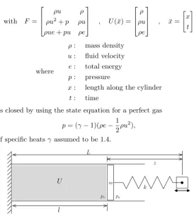
The model problem consists of a closed one-dimensional cylinder filled with gas, coupled to a spring–loaded piston. See Figure 4.1 for a schematic overview. The attachment point of the spring follows a prescribed, periodic motion. This model is similar to the one used in [1], but with the spring attached to a moving wall. The goal of this model problem is to mimic the qualitative behaviour of the CFD, CSD and trim procedures of a full rotorcraft simulation with a model that is as simple as possible. This model can then be used to analyse different coupling strategies.
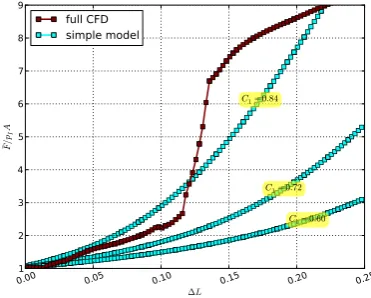
In the model problem the mass–spring system represents the CSD model for the rotor blades. The CFD model of the gas in the piston delivers a non-trivial force on the piston, analogous to how the complex aerodynamic forces deform the rotor blades in rotorcraft. The forced periodic motion of the spring attachment point induces a periodic solution of the combined fluid-structure system. This represents the periodicity of steady forward flight conditions. The trimming process is modelled by adjusting the spring constant. This indirectly alters the motion of the piston and the aerodynamic forces exerted on it.
The model equations are presented in a space–time formulation and subsequently discretised with a finite volume approach. This is roughly based on the discontinuous Galerkin finite element method of Van der Vegt and Van der Ven[14]. An important advantage of this approach for rotorcraft modelling is that local mesh refinement can be done naturally for both the space and time dimensions, which is useful for capturing blade vortices. Furthermore, the periodicity requirement becomes just another boundary condition, which is useful for modelling rotorcraft in stationary flight. For the model problem, however, both advantages will not be used, in order to keep the numerical procedure simple.
4.1. Governing Equations
The fluid in the cylinder of lengthl(t) is described by the Euler equations of gas dynamics in conservative form, which in space–time formulation can be written as:
with F=
ρu ρ
ρu2+p ρu
ρue+pu ρe
, U(¯x) = ρ ρu ρe
, x¯= "
x
t #
where
ρ: mass density u: fluid velocity e: total energy p: pressure
x: length along the cylinder t: time
This system is closed by using the state equation for a perfect gas p= (γ−1)(ρe−1
2ρu
2),
with the ratio of specific heatsγ assumed to be 1.4.
k
ps pa
m
U
l
L
[image:26.595.146.421.75.392.2]z
Figure 4.1.:Piston model problem
The structure is modelled with an ordinary differential equation describing a mass–spring system with one degree of freedom:
S: m( ¨L+ ¨z) +kz= (ps−pa)A. (4.2)
Here z is the displacement of the structure relative to the spring equilibrium position, in the same direction as L, so a positive ˙z means an increasing cylinder volume. m is the mass of the piston,kthe spring constant andA the surface area of the piston. The forcing term of the spring equation is the difference of the force exerted by the fluid on the pistonpsAand the force
resulting from the atmospheric pressurepaAoutside the cylinder.
To describe the motion of the wall the spring is attached to, the equilibrium position is a prescribed function of timeL(t). The motion is chosen to be a simple sinusoidal with periodtL,
mean value ¯Land amplitude ∆L.
L(t) = ¯L+ ∆Lcos (ωLt),
with ωL=
2π tL
4.1.1. Boundary conditions and model coupling
At the fluid–structure interface conservation of mass, momentum and energy is satisfied by the following dynamic and kinematic conditions.
FΓ≡ pΓ l uΓ = ps
L+z ˙ L+ ˙z
≡ SΓ (4.3)
The variablespΓ anduΓ denote the fluid pressure and velocity at the fluid–structure boundary.
Together (4.1), (4.2) and (4.3) describe the coupled fluid–structure system.
Due to the forced motion of the spring attachment point, work is done by the piston on the gas. This work results in a net increase of energy in the fluid system. In order to obtain a periodic solution the total internal energy of the system must be bounded. To this end the left wall is kept at a fixed temperature. The moving right wall is modelled as an adiabatic wall, as this results in a simpler boundary condition than the isothermal wall. The idea of this setup is that energy added to the gas by the work of the piston can leave the system at the isothermal left wall as an outward heat flux.
For S initial conditions zI and ˙zI are given. F can either have an initial condition or a
periodicity requirement. For the model problem an initial condition is prescribed by the fluid state that is defined by the parametersρI, uI,pI.
4.1.2. Nondimensionalisation
All the variables and equations are nondimenionalised. The reference quantities for the scaling are derived from the length ¯L, density ρI and pressure pI. Additionally, the fluid variables
are scaled with the cylinder cross-section area A, such that Equation (4.1) describes the fluid system in one-dimensional form. No new notation will be introduced, but instead all variables are assumed nondimensional from now on. All relevant variables are listed in Table A.2 and the dimensional values of the parameters are listed in Table A.1.
4.2. Fluid discretisation
The fluid is discretised using a space–time finite volume approach. In the time direction the space-time domain is partitioned in evenly spaced space–time slabs of height ∆t. The domain Ω for the space–time slabt∈[t0, t1] is depicted in Figure 4.2. The motion of the right boundary is
linearly interpolated between the valuesl0=l(t0) andl1=l(t1).
Along the spatial direction, Ω is divided into N evenly distributed elements. The length of an element in thex-direction ish0 =l0/N and h1 =l1/N at time t0 and t1 respectively. The
element boundary ∂Ωi is divided into four parts. S− and S+ are the time boundaries of the
element, at timet0andt1respectively andSi−1andSi are the left and right boundary, internal
to the space–time slab.
Ω:
Ω1 ΩNS−
h1
t0
t1
∆
t
h0 l
0 l1
S+
∆xi
Si
Si−1
Ωi
x
t
Figure 4.2.:Fluid discretisation in one space–time slab
To construct the finite volume discretisation Equation (4.1) is integrated over an element Ωi
and the divergence theorem is applied. This results in 0 =
Z
Ωi
∇ ·F(U)dΩ
= Z
∂Ωi
F(U)·¯n dS
with ¯nthe unit outward space–time normal vector of the element boundary.
The length of each part of the boundary and the unit normal vector pointing in the positivet direction forS−, S+ and in the positivexdirection forSi are given by
kS−k=h0 kS+k=h1 kSik=
q
∆t2+ ∆x2
i
¯
n−= ¯n+=
" 0 1 #
¯ ni=
" ∆t
−∆xi
# 1
kSik .
The integral over the element boundary ∂Ωi can now be split into four parts. If F(U) is
assumed to have a unique value FS, constant on each of element boundary parts, the surface
integral can be reduced to Z
∂Ωi
F(U)·n dS¯ = Z
S+
F(U)·ndS¯ + Z
S−
F(U)·ndS¯ + Z
Si
F(U)·ndS¯ + Z
Si−1
F(U)·ndS¯
= Z
S+
FS+·n¯+dS− Z
S−
FS−·n¯−dS+ Z
Si
FSi·n¯idS−
Z
Si−1
FSi−1·n¯i−1dS =FS+·n¯+kS+k −FS−·n¯−kS−k+FSi·¯nikSik −FSi−1·n¯i−1kSi−1k. (4.4)
4.2.1. Numerical flux
AsU is not uniquely defined at the element boundarySj the fluxF(U) can not directly be used
in (4.4) as the value ofFS. Instead a numerical flux is introduced. For the purpose of this model
problem, with the flow state assumed constant in an element, a simple Rusanov flux, as described by Toro[15], will suffice. This flux is used at every part of the element boundary. The left state UL is the state inside the element and the right stateUR the state in the adjacent element.
FS·n¯uH(UL, UR,n¯)
= 1
2(F(UL) +F(UR))·n¯+ 1
2(UL−UR)¯λ,
with λ¯= max(¯λL,¯λR) ¯λL/R = max
u 1
u−a 1
u+a 1
·¯n
a=pγp/ρ
The numerical flux is conservative, i.e.H(UL, UR,n¯) = −H(UR, UL,−n¯), so it can be used in
(4.4).
At the element boundaries between the different space–time slabs,S− andS+, this numerical
flux yields
FS−·n¯=U
t0
Ωi , FS+·n¯=UΩi,
withUt0
Ωi the value ofU at element Ωi in the previous space–time slab.
At the interior boundary parts in the space–time slab, Si, the flux is
FSi·n¯ =Hi with Hi=H(UΩi, UΩi+1,n¯) fori= 1, . . . , N−1.
Fori= 0, N the fluxHi must come from the boundary conditions.
Applying the expressions for FS·¯nin (4.4) and rewriting them using ˆHi=HikSik∆t−1 and
ˆ
λ= ¯λkSik∆t−1 yields the following equation for each element Ωi. h1UΩi−h0U
t0
Ωi+ ∆t
ˆ
Hi−Hˆi−1
= 0 (4.5)
with Hˆi=
1
2(F(UL) +F(UR))· "
1
−v #
+1
2(UL−UR)ˆλ, ˆ
λ= max |uL−v|+aL
|uR−v|+aR
!
, v= ∆xi
∆t
Here the wave speed ˆλ used in the approximate solution of the Riemann problem is an upper bound of the characteristic wave speeds, as described in [15]. Note how the length of the boundary cancels with the scaling of the normal and how the inner product with ¯nin the equation for ¯λ results in the correction of the fluid velocity with the element boundary velocity.
4.2.2. Boundary conditions
At the left and right boundaries of Ω a solid wall is assumed. On the left side of the domain the wall is stationary and on the right side the wall is moving. Given the velocity v = ∆∆xt of the wall and the flow stateU at the wall, the exact flux at the left and right boundaries of the space–time slab can be calculated
F(U)·n¯=F(U)·
" ∆t
−∆xi
# 1
kSik
=F(U)·
" 1
−v #
∆t
kSik
=
ρu−ρv
ρu2+p−ρuv ρue+pu−ρev
∆t
kSik
=
ρ(u−v) ρu(u−v) +p ρe(u−v) +pu
∆t
kSik .
With the requirement for the solid wall,u=v, the flux simplifies to
F(U)·n¯= 0 p pv ∆t
kSik
. (4.6)
This means that the only variable from the flow state that needs to be specified at the boundary is the pressure.
Right boundary: moving adiabatic wall
Because the length of the fluid domain is interpolated linearly betweenl0 andl1, the velocity of
the moving right wall,vr, is constant.
vr= l1−l0
In the case of an adiabatic wall, the pressure at the wall should be such that there is no heat transferred through the wall.
In a first attempt to achieve this, the pressure of the interior is simply extrapolated to the wall. With the notation used in describing a Riemann problem, wherepL denotes the pressure
in the element next to the wall andp∗ the pressure at the wall, this approach can be written as p∗=pL.
The results are however unsatisfactory. With increasing resolution of the space-time grid the particle velocity in the element adjacent to the wall does not converge to the speed of the wall.
A second approach for modelling an adiabatic moving wall is described by Toro[15]. The pressure comes from the solution of a Riemann problem where the left state is the state in the element next to the wall and the right state comes from a dummy element. If the left state is defined by ρL, uL and pL, then the dummy state is given by the conditions ρR =ρL, uR=−uL+ 2v andpR=pL. These particular left and right states allow the Riemann problem
to be solved analytically. The solution consists of either two shocks or two rarefaction waves. If local subsonic flow is assumed, the fluid state at the wall is the star state from the Riemann problem. The fluid velocity at the wall is thenu∗ = v, suggesting that the dummy state was chosen correctly to describe a wall moving with velocityv. The pressure at the wall is given by
p∗= pL
1 +γ−12 uL−v
aL
γ2−1γ
ifuL≤v, pL 1 +γγ+14
uL−v
aL
2 1 +
r
1 +γ+14 uL−v
aL
−2 !!
ifuL> v.
(4.7)
Using this pressure in (4.6) yields a numerical procedure that follows the prescribed velocity of the wall accurately.
Left boundary: fixed isothermal wall
Unfortunately, the flux associated with an isothermal boundary condition cannot be calculated as easily as for the case of an adiabatic wall. This is because the Riemann problem can not be solved analytically due to the fact thatpR 6=pL. In [16] an alternative approach based on the
approximate Riemann solver of Osher is suggested. A dummy state is constructed that, when used with the Osher solver, gives the desired properties at the wall (u∗= 0 andT∗=T∞). The
resulting pressure at the wall to be used in (4.6) is
p∗=pL
1 + γ−1 2
uL aL
1 + uL(a
2
L−a2∞)
aLa∞aLγ+−1a∞ +uL
a2
L+a2∞
2 2γ γ−1 .
The temperature requirement is expressed here as a prescribed speed of sounda∞. This speed
of sound is related to the temperature bya∞=pγRgasT∞, withRgas=cp−cv, the specific gas
constant. Notice the similarity of this expression forp∗to that of the adiabatic wall for the two rarefactions case withv= 0.
In testing this method, it was seen that the temperature at the wall was not reliably kept to a fixed value. Thus the approach of directly calculating the flux was abandoned for the isothermal left wall. Instead a dummy state is introduced and the numerical flux is calculated the same way
as at the internal element boundaries. The dummy stateU0 used in the numerical flux is defined
with
ρR=ρL ,
uL+uR
2 = 0 ,
TL+TR
2 =T∞.
Testing revealed that this implementation of the isothermal boundary condition was good in maintaining the prescribed temperature at the wall and adequate in prescribing a vanishing velocity at the fixed wall. The minor fluctuations of the fluid velocity at the fixed wall did not lead to a net mass flux through the boundary over a complete period.
Expressions for the boundary flux
The final boundary conditions can now be expressed in a way that they can be used in (4.5). The left isothermal boundary condition leads a dummy stateU0 that can be used in the numerical
flux procedure.
ˆ
H0= ˆH(U0, UΩ1)
with U0=
ρ1
−ρ1u1
ρ1e1+γ−12
p∞ρρ∞1 −p1
(4.8)
Hereρ1,u1,e1and p1 come fromUΩ1, the flow state in the leftmost internal element. The right adiabatic boundary condition leads to a direct expression of the flux:
ˆ HN =
0 p∗
p∗vr
, (4.9)
withp∗ from (4.7) andvr the velocity of the right moving wall, the piston.
4.2.3. Iterative solution strategy
Applying Equation (4.5) to every element in the space–time slab Ω results in a system of equa-tions. This system is to be solved for every space–time slab, analogous to time stepping in a classical finite volume approach with only a space dimension.
In order to solve the system described by (4.5), (4.8) and (4.9), a pseudo-time integration method is used. The quantity on the left hand side of (4.5) is called the residual, R. Finding the solution forR(U) = 0 then amounts to finding the stationary point of
∂U
∂τ +R(U) = 0. with R(U) =h1UΩi−h0U
t0
Ωi+ ∆t
ˆ
Hi−Hˆi−1
The stationary point can be found with an iterative procedure.
Un+1=Un−(∆τ)−1R(Un) (4.10) with ∆τ= h0+h1
2 + ∆tmax(ˆλi).
4.3. Structure discretisation
The pressure at the fluid–structure interface is assumed to be constant in a space–time slab, so if the forced motion of the springLis interpolated linearly on a space–time slab, Equation (4.2) can be solved analytically. The solutionz(t) has the general form
z(t) =α0sin (ω(t−t0)) +α1cos (ω(t−t0)) +β0+β1(t−t0),
with ω= r
k
m .
To satisfy the linear part of (4.2), the parametersβ0 andβ1must be
β0=
(ps−pa)A
k −
m k
¨ L(t0)
β1=−
m k
1 ∆t
¨
L(t1)−L¨(t0)
.
The remaining parametersα0 and α1 are used to satisfy the initial conditions z(t0) = z0 and
˙
z(t0) = ˙z0.
α0=
˙ z0−β1
ω α1=z0−β0
With these parameters known the values ofz and ˙z att=t1 can be calculated.
z1=z0cos (ω∆t) +
˙ z0
ω sin (ω∆t) +β0(1−cos(ω∆t)) +β1
∆t− 1
ωsin(ω∆t)
˙
z1= ˙z0cos (ω∆t)−ωz0sin (ω∆t) +β0ωsin (ω∆t) +β1(1−cos(ω∆t))
4.4. Coupling methods
The fluid, structure and trim procedures of the model problem will be coupled in a way similar to the coupling in the simulation of trimmed rotorcraft aeroelastics as described in Section 2.4.
4.4.1. Tight coupling
The approach shown in Figure 2.3 is based on a full space–time solver for bothFandS, i.e. the full periodic solution of eitherForS is calculated before information is exchanged. In the model problem explicit time stepping is used by solving each space–time slab separately. At each time step the models are coupled and information is exchanged. This is comparable to the tightly coupled procedure in rotorcraft simulations. By calculating a combined fluid–structure solution for a number of periods, a periodic solution is obtained without a specific periodic boundary condition.
Algorithm 1 gives an overview of how the systems are coupled. The goal is to find a periodic solution for the piston motion, a periodic fluid flow state and a value for the trim parameter T such that the average aerodynamic force on the piston, ¯F, is equal to some prescribed value Ftarget. At the end of each outer iteration the trim procedure T chooses a new valueTi+1 that
(hopefully) results in a better ¯Fi+1. The stopping criterionneed not be the same for the various
loops. The exact value used is not of importance to the current analysis, so it can be seen as a placeholder. The exact nature of the trim procedure and which parameter of the model it uses as the trim parameterT will be described in Section 4.5.
Algorithm 1: Tightly coupled procedure for solving the model problem initialise trim parameterT0; // guess
repeati= 1, . . . // (T loop)
t= 0 ;
z0=zI, ˙z0= ˙zI ;
initialise flow stateU0=UI ;
repeatj= 0, . . . // time stepping
initialisez0
1,z˙10 ; // guess repeatk= 1, . . . // S–F loop
Ujk =F(Uj−1, z0, z1k) ;
calculate pΓ from Ujk ; z1k+1,z˙1k+1=S(pΓ, z0,z˙0) ; until|zk
1 −z
k−1 1 |< ;
t=t+ ∆t; (z0,z˙0) = (z1,z˙1) ; untilpΓ periodic;
calculate ¯Fi from periodic solutionU ;
adjust trim: Ti+1=T(Ti,F¯i) ;
until|F¯i−Ftarget|< ;
4.4.2. Loose coupling
As shown in Figure 2.2, the basis of the loose coupling approach consists of the tight coupling with the CFD model replaced by a simplified model. Once the CSD and the simplified fluid model have converged to a trimmed periodic solution, the full CFD model is used to calculate a correction on this estimate. The input for this corrector step is a vectorzwith the displacement of the piston for one period. The result of the CFD model is used to construct a vector ∆p
which is the difference of the periodic pressure at the piston calculated by the simplified model and the CFD model.
∆p=pΓ−pΓˆ (4.11)
The variables written in a bold face denote a vector with lengthNt, the number of time steps in
one period.
Nt=tL/∆t
The pressure difference ∆pis then used in the next predictor step, where it is added to the pressure calculated by the simple model ˆpΓ. This result is the pressure from the fluid on the
pressureps.
ps=ˆpΓ+∆p (4.12)
Due to the addition∆pin the coupled procedure, the trim parameter needed to obtainFtarget
on the piston is close enough to the target value. The complete procedure is shown in Algorithm 2.
Algorithm 2: Loosely coupled procedure for solving the model problem initialise trim parameterT0; // guess
initialise∆p0(j) = 0 j= 0, . . . , Nt ;
repeatn= 1, . . . // F loop
repeati= 1, . . . // S–T loop
t= 0 ;
z0=zI, ˙z0= ˙zI ;
repeatj= 0, . . . // time stepping
initialisez0
1,z˙10 ; // guess
repeatk= 1, . . . // simplified S–F loop
calculate ˆpΓ with simplified model ;
ps= ˆpΓ+∆pn(jmodNt) ; z1k+1,z˙1k+1=S(ps, z0,z˙0) ; until|zk
1 −z
k−1 1 |< ;
t=t+ ∆t; (z0,z˙0) = (z1,z˙1) ; untilps periodic;
save complete period ofz0 and ˆpΓ in zn andˆpnΓ ;
calculate ¯Fi from periodic solutionps;
adjust trim: Ti+1=T(Ti,F¯i) ;
until|F¯i−Ftarget|< ; t= 0 ;
t= 0 ;
z0=zI, ˙z0= ˙zI ;
initialise flow stateU0=UI ;
repeatj= 0, . . . // time stepping
Uj=F(Uj−1,zn(j−1),zn(j)) ;
calculate pΓ from Ujk ;