Exponential Priors for Maximum Entropy Models
Joshua Goodman
One Microsoft Way
Redmond, WA 98052
j
[email protected]
Abstract
Maximum entropy models are a common mod-eling technique, but prone to overfitting. We show that using an exponential distribution as a prior leads to bounded absolute discounting by a constant. We show that this prior is better motivated by the data than previous techniques such as a Gaussian prior, and often produces lower error rates. Exponential priors also lead to a simpler learning algorithm and to easier to understand behavior. Furthermore, exponential priors help explain the success of some previ-ous smoothing techniques, and suggest simple variations that work better.
1
Introduction
Conditional Maximum Entropy (maxent) models have been widely used for a variety of tasks, including lan-guage modeling (Rosenfeld, 1994), part-of-speech tag-ging, prepositional phrase attachment, and parsing (Rat-naparkhi, 1998), word selection for machine translation (Berger et al., 1996), and finding sentence boundaries (Reynar and Ratnaparkhi, 1997). They are also some-times called logistic regression models, maximum likeli-hood exponential models, log-linear models, and are even equivalent to a form of perceptrons/single layer neural networks. In particular, perceptrons that use the standard sigmoid function, and optimize for log-loss are equivalent to maxent. Multi-layer neural networks that optimize log-loss are closely related, and much of the discussion will apply to them implicitly.
Conditional maxent models have traditionally either been unregularized or regularized by using a Gaussian prior on the parameters. We will show that by using an exponential distribution as the prior, several advantages can be gained. We will show that in at least one case, an exponential prior experimentally better matches the ac-tual distribution of the parameters. We will also show that it can lead to improved accuracy, and a simpler learning
algorithm. In addition, the exponential prior inspires an improved version of Good Turing discounting with lower perplexity.
Conditional maxent models are of the form
PΛ(y|x) = exp
F
i=1λifi(x, y)
yexp
iλifi(x, y)
wherexis an input vector,yis an output, thefiare the so-called indicator functions or feature values that are true if a particular property ofx, y is true,F is the number of such features,Λrepresents the parameter setλ1...λn, andλi is a weight for the indicator fi. For instance, if trying to do word sense disambiguation for the word “bank”,xwould be the context around an occurrence of the word;ywould be a particular sense, e.g. financial or river;fi(x, y)could be 1 if the context includes the word “money” andyis the financial sense; andλiwould be a large positive number.
Maxent models have several valuable properties (Della Pietra et al. (1997) give a good overview.) The most important is constraint satisfaction. For a givenfi, we can count how many times fi was observed in the training data with valuey, observed[i] = jfi(xj, yj). For a modelPΛwith parametersΛ, we can see how many times the model predicts that fi would be expected to occur: expected[i] = j,yPΛ(y|xj)fi(xj, y). Maxent models have the property that expected[i] = observed[i]
for alliandy. These equalities are called constraints. The next important property is that the likelihood of the training data is maximized (thus, the name maximum likelihood exponential model.) Third, the model is as similar as possible to the uniform distribution (minimizes the Kullback-Leibler divergence), given the constraints, which is why these models are called maximum entropy models.
infi-nite, even actual zero probabilities), and to exhibit other symptoms of severe overfitting. There have been a num-ber of approaches to this problem, which we will discuss in more detail in Section 3. The most relevant approach, however, is the work of Chen and Rosenfeld (2000), who implemented a Gaussian prior for maxent models. They compared this technique to most of the previously im-plemented techniques, on a language modeling task, and concluded that it was consistently the best. We thus use it as a baseline for our comparisons, and similar considera-tions motivate our own technique, an exponential prior.
Chen et al. place a Gaussian prior with 0 mean andσ2i variance on the model parameters (theλis), and then find a model that maximizes the posterior probability of the data and the model. In particular, maxent models without priors use the parametersΛthat maximize
arg max
Λ
n
j=1
PΛ(yj|xj)
wherexj, yjare training data instances. With a Gaussian prior we find
arg max
Λ
n
j=1
PΛ(yj|xj)×F
i=1
1
2πσ2
i exp
−λ2i 2σ2
i
In this case, a trained model does not satisfy the con-straints expected[i] = observed[i], but, as Chen and Rosenfeld show, instead satisfies constraints
expected[i] =observed[i]− λi
σ2
i
(1)
That is, instead of a model that matches the observed count, we get a model matching the observed count minus
λi
σ2
i: in language modeling terms, this is “discounting.” We do not believe that all models are generated by the same process, and therefore we do not believe that a single prior will work best for all problem types. In particular, as we will describe in our experimen-tal results section, when looking at one particular set of parameters, we noticed that it was not at all Gaus-sian, but much more similar to a 0 mean Laplacian,
f(λi) = 1 2βiexp
−|λi|
βi
, or to an exponential
distri-butionf(λi) =αiexp (−αiλi), which is non-zero only for non-negativeλi. In some cases, learned parameter distributions will not match the prior distribution, but in some cases they will, so it seemed worth exploring one of these alternate forms. Later, when we try to optimize our models, the parameter seach will turn out to be much simpler with an exponential prior, so we focus on that distribution.
With an exponential prior, we maximize
arg max
Λ≥0
n
j=1
PΛ(yj|xj)×F
i=1
αiexp (−αiλi) (2)
As we will describe, it is significantly simpler to perform this maximization than the Gaussian maximization. Fur-thermore, as we will describe, models satisfying Equa-tion 2 will have the property that, for each λi, either a) λi = 0 and expected[i] ≥ observed[i]−αi or b)
expected[i] =observed[i]−αi. In other words, we essen-tially just discount the observed counts by the constant
αi (which is the reciprocal of the standard deviation), subject to the constraint thatλiis non-negative. This is much simpler and more intuitive than the constraints with the Gaussian prior (Equation 1), since those constraints change as the values ofλi change. Furthermore, as we will describe in Section 3, discounting by a constant is a common technique for language model smoothing (Ney et al., 1994; Chen and Goodman, 1999), but one that has not previously been well justified; the exponential prior gives some Bayesian justification.
In Section 5 we will show that on two very different tasks – grammar checking and a collaborative filtering task – the exponential prior yields lower error rates than the Gaussian.
2
Learning algorithms and discounting
In this section we derive a learning algorithm for expo-nential priors, with provable convergence properties, and show that it leads to a simple discounting formula. Note that the simple learning algorithm is an important con-tribution: the algorithm for a Gaussian prior is quite a bit more complicated, and previous related work with the Laplacian prior (two-sided exponential) has had a diffi-cult time finding learning algorithms; because the Lapla-cian does not have a continuous first derivative, and be-cause the exponential prior is bounded at 0, standard gra-dient descent type algorithms may exhibit poor behav-ior. Williams (1995) devotes a full ten pages to describ-ing a somewhat heuristic approach for solvdescrib-ing this prob-lem, and even this discussion concludes “In summary it is left to the reader to supply the algorithms for deter-mining successive search directions and the initially pre-ferred value of” the step size (page 130).1 We show that a very simple variation on a standard algorithm, General-ized Iterative Scaling (GIS) (Darroch and Ratcliff, 1972), solves this problem. In particular, as we will show, while GIS uses an update rule of the form
λi:=λi+ 1 f#log
observed[i] expected[i]
1
our modified algorithm uses a rule of the form
λi:= max
0,
λi+ 1 f#log
observed[i]−αi expected[i]
(3) Note that there are two different styles of model that one can use, especially in the common case that there are two outputs (values fory.) Consider a word sense disam-biguation problem, trying to determine whether a word like “bank” means the river or financial sense, with ques-tions like whether or not the word “water” occurs nearby. One could have a single indicator functionf1(x, y) =
1 if water occurs nearby and values in the range−∞<
λ1 < ∞. We call this style “double sided” indicators. Alternatively, one could have two indicator functions,
f1(x, y) = 1 if water occurs nearby and y=river and
f2(x, y) = 1 if water occurs nearby and y=financial. In
this case, one could allow either−∞< λ1, λ2 <∞or
0 ≤λ1, λ2 <∞. We call the style with two indicators “single sided.” With a Gaussian prior, it does not mat-ter which style one uses – one can show that by chang-ingσ2, exactly the same results will be achieved. With a Laplacian (double sided exponential), one could also use either style. With an exponential prior, only positive val-ues are allowed, so one must use the double sided style, so that one can learn that some indicators push towards one sense, and some push towards the other – that is, rather than having one weight which is positive or neg-ative, we have two weights which are positive or zero, one of which pushes towards one answer, and the other pushing towards the other.
We derive our constraints and learning algorithm by very closely following the derivation of the algorithm by Chen and Rosenfeld. It will be convenient to maximize the log of the expression in 2 rather than the expression itself. This leads to an objective function:
L(Λ) =
j
logPΛ(yj|xj)−F
i=1
αiλi+ logαi
=
j F
i=1
λifi(xj, yj) (4)
−
j log
y
exp F i=1
λifi(xj, y)
−F
i=1
αiλi+logαi
Note that this objective function is convex (since it is the sum of two convex functions.) Thus, there is a global maximum value for this objective function.
Now, we wish to find the maximum. Normally, we would do this by setting the derivative to 0, but the bound ofλk ≥0changes things a bit. The maximum can then occur at the discontinuity in the derivative (λk = 0) or whenλk >0. We can explicitly check the value of the objective function at the pointλk = 0. When there is a
maximum withλk >0we know that the partial deriva-tive with respect toλkwill be 0.
∂ ∂λk
j
F
i=1λifi(xj, yj)
−jlogyexpiF=1λifi(xj, y)
−Fi=1αiλi+const(Λ)
= jfk(xj, yj)
−j
yfk(xj,y) exp(
F
i=1λifi(xj,y))
yexp
F
i=1λifi(xj,y)
−αk =jfk(xj, yj)−jyfk(xj, y)PΛ(y|xj)−αk
This implies that at the optimum, whenλk>0,
j
fk(xj, yj)−
j
y
fk(xj, y)PΛ(y|xj)−αk= 0
observed[k]−expected[k]−αk = 0
observed[k]−αk =expected[k] (5)
In other words, we discount the observed count byαk– the absolute discounting equation. Sometimes it is better forλk to be set to 0 – another possible optimal point is whenλk = 0and observed[k]−αk <expected[k]. One of these two cases must hold at the optimum.
Notice an important property of exponential priors (analogous to a similiar property for Laplace priors (Williams, 1995; Tibshirani, 1994)): they often favor pa-rameters that are exactly 0. This leads to a kind of natu-ral pruning for exponential priors, not found in Gaussian priors, which are only very rarely 0. (Note, however, that one should not increase theα’s in the exponential prior to control pruning, as this may lead to oversmoothing. If additional pruning is needed for speed or memory sav-ings, feature selection techniques should be used, such as pruning small or infrequent parameters, instead of a strengthened prior.)
Now, we can derive the update equations. The deriva-tion is exactly the same as Chen and Rosenfeld’s (2000) with the minor change of an exponential prior instead of a Gaussian prior (we include it in the appendix.) Let
f#(x, y) =
ifi(x, y). Then, in the end, we get an
update equation of the form
λk:= max
0, λk+ 1 f#log
observed[k]−αk expected[k]
Compare this equation to the corresponding equation with a Gaussian prior (Chen and Rosenfeld., 2000). With a Gaussian prior, one can derive an equation of the form
observed[k]−λk
σ2
k
=expected[k] expf#δk
One can also derive variations on this update. For in-stance, in the Appendix, we derive an update for Im-proved Iterative Scaling (Della Pietra et al., 1997) with an exponential prior. Perhaps more importantly, one can also derive updates for Sequential Conditional General-ized Iterative Scaling (SCGIS) (Goodman, 2002), which is several times faster than GIS. The SCGIS update for binary features with an exponential prior is simply
λk:= max
0, λk+ logobserved[k]−αk
expected[k]
One might wonder why we simply don’t use conju-gate gradient (CG) methods, which have been shown to converge quickly for maxent. There has not been a for-mal comparison of SCGIS to conjugate gradient methods. In our own pilot studies, SCGIS is sometimes faster and sometimes slower. Also, some versions of CG use heuris-tics for the step size, and lose convergence guarantees. Finally, SCGIS is simpler to implement than conjugate gradient, and even for those with a conjugate gradient li-brary, because of the parameter constraints (for an expo-nential prior) or discontinuous derivatives (for a Lapla-cian) standard conjugate gradient techniques need to be at least somewhat modified.
Good-Turing discounting has been used or suggested for language modeling several times (Rosenfeld, 1994, page 38), (Lau, 1994). In particular, it has been suggested to use an update of the form
λk :=λk+ 1 f#log
observed[k]∗ expected[k]
where observed[k]∗is the Good-Turing discounted value of observed[k]. This update has a problem, as noted by its proponents: the constraints are probably now inconsistent – there is no model that can simultaneously satisfy them. We note that a simple variation on this update, inspired by the exponential prior, does not have these problems:
λk := max 0,
λk+ 1 f#log
observed[k]∗ expected[k]
In particular, this can be thought of as picking an
αobserved[k] for each observed[k]. This does not con-stitute a Bayesian prior, since the value is picked after the counts are observed, but it does lead to a convex objective function with a global maximum, and the update function will converge towards this maximum. Variations on the constraints of Equation 5 will apply for this modified ob-jective function. Furthermore, in the experimental results section, we will see that on a language modeling task, this modified update function outperforms the traditional update. By using a well motivated approach inspired by exponential priors, we can find a simple variation that has better performance both theoretically and empirically.
3
Previous Work
There has been a fair amount of previous work on regu-larization of maxent models. Early approaches focused on feature selection (Della Pietra et al., 1997) or, simi-larly, count cutoffs (Rosenfeld, 1994). By not using all features, there is typically extra probability left-over for unobserved events, which is distributed in a maximum entropy fashion. The problem with this approach is that it ignores useful information – although low count or low discrimination features may cause overfitting, they do contain valuable information. Because of this, more re-cent approaches (Rosenfeld, 1994, page 38), (Lau, 1994) have tried techniques such as Good-Turing discounts (Good, 1953).
There are a number of other approaches (Khudanpur, 1995; Newman, 1997) based on the fuzzy maxent frame-work (Della Pietra and Della Pietra, 1993). Chen and Rosenfeld (Chen and Rosenfeld., 2000) give a more com-plete discussion of those approaches.
Chen and Rosenfeld (2000), following a suggestion of Lafferty, implemented a Gaussian prior for maxent mod-els. They compared this technique to most of the previ-ously discussed techniques, on a language modeling task, and concluded that it was consistently the best technique. Tibshirani (1994) introduced Laplacian priors for lin-ear models (linlin-ear regressions) and showed that an ob-jective function that minimizes the absolute values of the parameters corresponds to a Laplacian prior. He called this the Least Absolute Shrinkage and Selection Operator (LASSO) and showed that it leads to a type of feature se-lection. Exponential priors are sometimes called single-sided Laplacians, so obviously, the two techniques are very closely related, so closely that we would not want to claim that either was better than the other.
Williams (1995) introduced a Laplacian prior for neu-ral networks. Single layer neural networks with cer-tain loss functions are equivalent to logistic regres-sion/maximum entropy models. Williams’ algorithm was for a more general case, and much more complex than the one we describe.
More recently, Figueiredo et al. (2003) in unpublished independent work also examined Laplacian priors for lo-gistic regression, deriving a somewhat more complex al-gorithm than ours, but one that they extended to partially supervised learning. He has shown that the results are comparable to transductive SVMs.
Perkins and Theiler (2003) used logisitic regression with a Laplacian prior as well. Their learning algorithm was conjugate gradient descent. Normally, conjugate gra-dient methods are only used on data that has a continuous first derivative, so the code was modified to prune weights that go exactly to zero.
priors with logistic regression, nor even the first good learning algorithm for the model type. Our contributions are performing an explicit comparison to a Gaussian prior and showing improved performance on real data; noticing that the fixed point of the models leads to absolute dis-counting; showing that iterative-scaling style algorithms including GIS, IIS, and SCGIS can be trivially modified to use this prior; and explicitly showing that in at least one case, parameters are actually consistent with this prior.
4
Kneser-Ney smoothing
In this section, we help explain the excellent performance of Kneser-Ney smoothing, the best performing language model smoothing technique. This justification not only answers an important question – why do discounting methods work well – but also gives guidance for extend-ing Kneser-Ney smoothextend-ing to problems with fractional counts, where solutions were not previously known.
Chen and Goodman (1999) performed an extensive comparison of different smoothing (regularization) tech-niques for language modeling. They found that a ver-sion of Kneser-Ney smoothing (Kneser and Ney, 1995) consistently was the best performing technique. Unfortu-nately, while there are partial theoretical justifications for Kneser-Ney smoothing, in terms of preserving marginals, one important part has previously had no justification: Kneser-Ney smoothing discounts counts, while most con-ventional regularization techniques, justified by Dirichlet priors, add to counts. Given that discounting was pre-viously unjustified, it is exciting that we have found a way to explain it. In fact, we can show that the Back-off version of Kneser-Ney smoothing is an excellent ap-proximation to a maximum entropy model with an ex-ponential prior. In particular, Kneser-Ney smoothing is derived by assuming absolute discounting, and then find-ing the distribution that preserves marginals, i.e. mak-ing expected = observed - discount. The differences be-tween Backoff Kneser-Ney smoothing and maxent mod-els with exponential priors are twofold. First, the backoff version does not exactly preserve marginals – an approx-imation is made. Second, Backoff Kneser-Ney always performs discounting, even when this effectively results in lowering the probability, e.g. the equivalent of a neg-ative value for λ.There is also an interpolated version of Kneser-Ney smoothing. The interpolated version of Kneser Ney smoothing works even better. It exactly pre-serves marginals (except for discounting.) Also, the sec-ondary distribution is combined with the primary distri-bution; this has several effects, including that it is un-likely to get the equivalent of a large negativeλvalue.
5
Experimental Results
In this section, we detail our experimental results, show-ing that exponential priors outperform Gaussian priors on two different data sets, and inspire improvements for a third. For all experiments, except the language model ex-periments, we used a single variance for both the Gaus-sian and the exponential prior, rather than one per param-eter, with the variance optimized on held out data. For the language modeling experiments, we used three variances, one each for the unigram, bigram, and trigram models, again optimized on held out data.
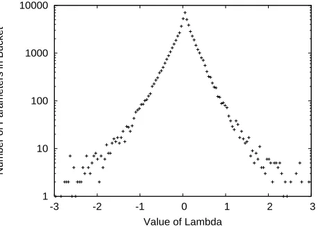
We were inspired to use an exponential prior by an actual examination of a data set. In particular, we used the grammar-checking data of Banko and Brill (2001). We chose this set because there are commonly used ver-sions both with small amounts of data (which is when we expect the prior to matter) and with large amounts of data (which is required to easily see what the distribu-tion over “correct” parameter values is.) For one exper-iment, we trained a model using a Gaussian prior, using a large amount of data. We then found those parameters (λ’s) that had at least 35 training instances – enough to typically overcome the prior and train the parameter re-liably. We then graphed the distribution of these param-eters. While it is common to look at the distribution of data, the NLP and machine learning communities rarely examine distributions of model parameters, and yet this seems like a good way to get inspiration for priors to try, using those parameters with enough data to help guess the priors for those with less, or at least to determine the correct form for the prior, if not the exact values.2 The results are shown in Figure 1, which is a histogram ofλ’s with a given value. If the distribution were Gaussian, we would expect this to look like an upside-down parabola. If the distribution were Laplacian, we would expect it to appear as a triangle (the bottom formed from the X-axis.) Indeed, it does appear to be roughly triangular, and to the extent that it diverges from this shape, it is convex, while a Gaussian would be concave. We don’t believe that the exponential prior is right for every problem – our argu-ment here is that based on both better accuracy (our next experiment) and a better fit to at least some of the param-eters, that the exponential prior is better for some models. We then tried actually using exponential priors with this application, and were able to demonstrate
improve-2Of course, those parameters with lots of data might be
1 10 100 1000 10000
-3 -2 -1 0 1 2 3
Number of Parameters in Bucket
[image:6.612.70.299.38.202.2]Value of Lambda
Figure 1: Histogram ofλvalues
ments in error rate. We used a small data set, 100,000 sentences of training data and ten different confusable word pairs. (Most training sentences did not contain ex-amples of the confusable word pairs of interest, so the actual number of training examples for each word-pair was less than 100,000). We tried different priors for the Gaussian and exponential prior, and found the best single prior on average across all ten pairs. With this best setting, we achieved a 14.51% geometric average error rate with the exponential prior, and 15.45% with the Gaussian. To avoid any form of cheating, we then tried 10 different word pairs (the same as those used by Banko and Brill (2001)) with this best parameter setting. The results were 18.07% and 19.47% for the exponen-tial and Gaussian priors respectively. (The overall higher rate is due to the test set words being slightly more dif-ficult.) We also tried experiments with 1 million and 10 million words, but there were not consistent differences; improved smoothing mostly matters with small amounts of training data.
We also tried experiments with a collaborative-filtering style task, television show recommendation, based on Nielsen data. The dataset used, and the definition of a col-laborative filtering (CF) score is the same as was used by Kadie et al. (2002), although our random train/test split is not the same, so the results are not strictly comparable. We first ran experiments with different priors on a held-out section of the training data, and then using the single best value for the prior (the same one across all features), we ran on the test data. With a Gaussian prior, the CF score was 42.11, while with an exponential prior, it was 45.86, a large improvement.
Finally, we ran experiments with language modeling, with mixed success. We used 1,000,000 words of train-ing data (a small model, but one where smoothtrain-ing mat-ters) from the WSJ corpus and a trigram model with a
cluster-based speedup (Goodman, 2001). We evaluated on test data using the standard language modeling mea-sure, perplexity, where lower scores are better. We tried five experiments: using Katz smoothing (a widely used version of Good-Turing smoothing) (perplexity 238.0); using Good Turing discounting to smooth maxent (per-plexity 224.8); using our variation on Good-Turing, in-spired by exponential priors, whereλ’s are bounded at 0 (perplexity 204.5); using an exponential prior (perplex-ity 190.8); using a Gaussian prior (perplex(perplex-ity 183.7); and using interpolated modified Kneser-Ney smoothing (per-plexity 180.2). On the one hand, an exponential prior is worse than a Gaussian prior in this case, and modified in-terpolated Kneser-Ney smoothing is still the best known smoothing technique (Chen and Goodman, 1999), within noise of a Gaussian prior. On the other hand, searching for parameters is extremely time consuming, and Good-Turing is one of the few parameter-free smoothing meth-ods. Of the three Good-Turing smoothing methods, the one inspired by exponentials priors was the best.
Note that perplexity is 2entropy and in general, we have found that exponential priors work slightly worse on entropy measures than the Gaussian prior, even when they are better on accuracy. This may be due to the fact that an exponential prior “throws away” some informa-tion, whenever theλwould be negative. (In a pilot exper-iment with a variation that does not throw away informa-tion, the entropies are closer to the Gaussian.)
6
Conclusion
We have shown that an exponential prior for maxent mod-els leads to a simple update formula that is easy to im-plement, and to models that are easy to understand: ob-servations are discounted, subject to the constraint that
λ ≥ 0. We have also shown that in at least one case, this prior better matches the underlying model, and that for two applications, it leads to improved accuracy. The prior also inspired an improved version of Good-Turing smoothing with lower perplexity. Finally, an exponential prior explains why models that discount by a constant can be Bayesian, giving an alternative to Dirichlet pri-ors which add a constant. This helps justify Kneser-Ney smoothing, the best performing smoothing technique in language modeling. In the future, we would like to use our technique of examining the distribution of model pa-rameters to see if other problems exhibit other priors be-sides Gaussian and Laplacian/exponential, and if perfor-mance on those problems can be improved through this observation.
Acknowledgments
pa-per. Finally, thanks to Stan Chen and Roni Rosenfeld: our derivation for exponential priors closely follows the text of their derivation for Gaussian priors.
References
M. Banko and E. Brill. 2001. Mitigating the paucity of data problem. In HLT.
Adam L. Berger, Stephen A. Della Pietra, and Vincent J. Della Pietra. 1996. A maximum entropy approach to natural language processing. Computational
Linguis-tics, 22(1):39–71.
Stanley F. Chen and Joshua Goodman. 1999. An empir-ical study of smoothing techniques for language mod-eling. Computer Speech and Language, 13:359–394, October.
Stanley Chen and Ronald Rosenfeld. 2000. A survey of smoothing techniques for ME models. IEEE Trans. on
Speech and Audio Processing, 8(2):37–50, January.
J.N. Darroch and D. Ratcliff. 1972. Generalized iterative scaling for log-linear models. The Annals of
Mathe-matical Statistics, 43:1470–1480.
Stephen Della Pietra and Vincent Della Pietra. 1993. Sta-tistical modeling by maximum entropy. Unpublished Manuscript.
Stephen Della Pietra, Vincent Della Pietra, and John Laf-ferty. 1997. Inducing features of random fields. IEEE
Transactions on Pattern Analysis and Machine Intelli-gence, 19(4):380–393, April.
Mario A. T. Figueiredo, Balaji Krishnapuram, Lawrence Carin, and Alexander J. Hartemink. 2003. Supervised and semi-supervised sparse Bayesian classification.
I.J. Good. 1953. The population frequencies of species and the estimation of population parameters.
Biometrika, 40(3 and 4):237–264.
Joshua Goodman. 2001. Classes for fast maximum en-tropy training. In ICASSP 2001.
Joshua Goodman. 2002. Sequential conditional general-ized iterative scaling. In ACL ’02.
Carl M. Kadie, Christopher Meek, and David Hecker-man. 2002. CFW: A collaborative filtering system using posteriors over weights of evidence. In
Proceed-ings of UAI, pages 242–250.
S. Khudanpur. 1995. A method of maximum entropy es-timation with relaxed constraints. In 1995 Johns
Hop-kins University Language Modeling Workshop.
Reinhard Kneser and Hermann Ney. 1995. Im-proved backing-off for m-gram language modeling. In
ICASSP, volume 1, pages 181–184.
Raymond Lau. 1994. Adaptive statistical language mod-elling. Master’s thesis, MIT.
W. Newman. 1997. Extension to the maximum en-tropy method. IEEE Trans. on Information Theory, IT-23(1):89–93, January.
Hermann Ney, Ute Essen, and Reinhard Kneser. 1994. On structuring probabilistic dependences in stochastic language modeling. Computer, Speech, and Language, 8:1–38.
Simon Perkins and James Theiler. 2003. Online feature selection using grafting. August.
Adwait Ratnaparkhi. 1998. Maximum Entropy Models
for Natural Language Ambiguity Resolution. Ph.D.
thesis, University of Pennsylvania.
J. Reynar and A. Ratnaparkhi. 1997. A maximum en-tropy approach to identifying sentence boundaries. In
ANLP.
Ronald Rosenfeld. 1994. Adaptive Statistical Language
Modeling: A Maximum Entropy Approach. Ph.D.
the-sis, Carnegie Mellon University, April.
Robert Tibshirani. 1994. Regression shrinkage and se-lection via the lasso. Technical report.
Peter M. Williams. 1995. Bayesian regularization and pruning using a Laplace prior. Neural Computation, 7:117–143.
A
Derivation of Update Equation
In each iteration, we try to find∆ ={δi}that maximizes the increase in the objective function (subject to the con-straint thatδi+λi≥0). From Equation 4,
L(Λ + ∆)−L(Λ) =
j
i
δifi(xj, yj)
−
j
log y
PΛ(y|xj) exp i
δifi(xj, y)
−
i αiδi
As with the Gaussian prior, it is not clear how to maxi-mize this function directly, so instead we use an auxiliary function,B(∆), with three important properties: first, we can maximize it; second, it bounds this function from be-low; third, it is larger than zero wheneverΛis not at a lo-cal optimum, i.e. does not satisfy the constraints in Equa-tion 5. Using the well-known inequalitylogx≤x−1, which implies−logx≥1−x, we get
j
i
δifi(xj, yj)
+
j 1−
y
PΛ(y|xj) exp i
δifi(xj, y)
−
i
αiδi (6)
Letf#(x, y) =ifi(x, y). Modify Equation 6 to:
LX(Λ + ∆)−LX(Λ)≥
j
i
δifi(xj, yj)+
j
1−
y
PΛ(y|xj) exp f#(x
j, y)
i
δi fi(xj, y) f#(xj, y)
−
i
αiδi (7)
Now, recall Jensen’s inequality, which states that for a convex functiong,
y
p(x)g(x)≥g
x p(x)x
Notice thatff#i((x,yx,y))is a probability distribution. Thus, we get
LX(Λ + ∆)−LX(Λ)≥
j
i
δifi(xj, yj)+
j
1−
y
PΛ(y|xj) i
fi(xj, y) f#(xj, y)exp
f#(x
j, y)δi
−
i
αiδi (8)
Now, we would like to find∆that maximizes Equation 8. Thus, we take partial derivatives and set them to zero, remembering to also check whether a maximum occurs whenδk= 0.
∂ ∂δk j i
δifi(xj, yj) + j
1
−
y
PΛ(y|xj) i
fi(xj, y) f#(xj, y)exp
f#(x
j, y)δi−
i αiδi
=
j
fk(xj, yj)
+
j
−
y
PΛ(y|xj)fk(xj, y) f#(xj, y)
∂ ∂δkexp
f#(x
j, y)δk−αk
=
j
fk(xj, yj)
−
j
y
PΛ(y|xj)fk(xj, y) expf#(x
j, y)δk−αk
= 0
This gives us a version of Improved Iterative Scaling with an exponential Prior. In general, however, we prefer vari-ations of Generalized Iterative Scaling, which may not converge as quickly, but lead to simpler algorithms. In particular, we setf#= maxx,yf#(x, y). Then, instead of Equation 7, we get
LX(Λ + ∆)−LX(Λ)
≥
j
i
δifi(xj, yj) +
j
1−
y
PΛ(y|xj) exp f#
i
δifi(xj, y) f#
−
i
αiδi (9)
We can follow essentially the same derivation from there. (Technically, we need to add in a slack parameter; the slack parameter can then be given a near-zero variance prior so that its value stays at 0, and thus in practice it can be ignored.) We thus get:
∂ ∂δk j i
δifi(xj, yj)+
j
1−
y
PΛ(y|xj) i
fi(xj, y)
f# exp f#δi−
i αiδi
=
j
fk(xj, yj)
−
j
y
PΛ(y|xj)fk(xj, y) expf#δ
k−αk
= observed[k]−expected[k] expf#δk−αk
= 0 (10)
From Equation 10 we get
δk = 1 f#log
observed[k]−αk expected[k]
Now,δk+λk may be less than 0; in this case, an illegal new value forλk would result. We know, however, from the monotonicity of all the equations with respect toδk that the lowest legal value ofδk will be the best, and we thus arrive at
δk= max
−λk, 1 f#log
observed[k]−αk expected[k]
or equivalently
λk:= max
0, λk+ 1 f#log
observed[k]−αk expected[k]