Training Tree Transducers
Jonathan Graehl
Information Sciences Institute
University of Southern California
4676 Admiralty Way
Marina del Rey, CA 90292
[email protected]
Kevin Knight
Information Sciences Institute
University of Southern California
4676 Admiralty Way
Marina del Rey, CA 90292
[email protected]
Abstract
Many probabilistic models for natural language are now written in terms of hierarchical tree structure. Tree-based modeling still lacks many of the standard tools taken for granted in (finite-state) string-based modeling. The theory of tree transducer automata provides a possible frame-work to draw on, as it has been frame-worked out in an extensive literature. We motivate the use of tree transducers for natural language and address the training problem for probabilistic tree-to-tree and tree-to-tree-to-string transducers.
1
Introduction
Much of natural language work over the past decade has employed probabilistic finite-state transducers (FSTs) operating on strings. This has occurred somewhat under the influence of speech recognition, where transducing acoustic sequences to word sequences is neatly captured by left-to-right stateful substitution. Many conceptual tools exist, such as Viterbi decoding (Viterbi, 1967) and forward-backward training (Baum and Eagon, 1967), as well as generic software toolkits. Moreover, a surprising variety of problems are attackable with FSTs, from part-of-speech tagging to letter-to-sound conversion to name transliteration.
However, language problems like machine transla-tion break this mold, because they involve massive re-ordering of symbols, and because the transformation pro-cesses seem sensitive to hierarchical tree structure. Re-cently, specific probabilistic tree-based models have been proposed not only for machine translation (Wu, 1997; Alshawi, Bangalore, and Douglas, 2000; Yamada and Knight, 2001; Gildea, 2003; Eisner, 2003), but also for
This work was supported by DARPA contract F49620-00-1-0337 and ARDA contract MDA904-02-C-0450.
summarization (Knight and Marcu, 2002), paraphras-ing (Pang, Knight, and Marcu, 2003), natural language generation (Langkilde and Knight, 1998; Bangalore and Rambow, 2000; Corston-Oliver et al., 2002), and lan-guage modeling (Baker, 1979; Lari and Young, 1990; Collins, 1997; Chelba and Jelinek, 2000; Charniak, 2001; Klein and Manning, 2003). It is useful to understand generic algorithms that may support all these tasks and more.
(Rounds, 1970) and (Thatcher, 1970) independently introduced tree transducers as a generalization of FSTs. Rounds was motivated by natural language. The Rounds tree transducer is very similar to a left-to-right FST, ex-cept that it works top-down, pursuing subtrees in paral-lel, with each subtree transformed depending only on its own passed-down state. This class of transducer is often nowadays called R, for “Root-to-frontier” (Gécseg and Steinby, 1984).
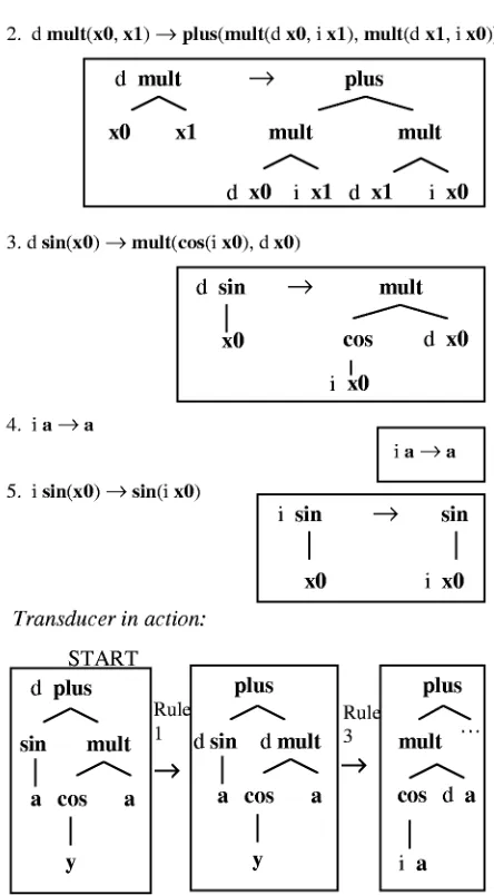
Rounds uses a mathematics-oriented example of an R transducer, which we summarize in Figure 1. At each point in the top-down traversal, the transducer chooses a production to apply, based only on the current state and the current root symbol. The traversal continues until there are no more state-annotated nodes. Non-deterministic transducers may have several productions with the same left-hand side, and therefore some free choices to make during transduction.
An R transducer compactly represents a potentially-infinite set of input/output tree pairs: exactly those pairs (T1, T2) for which some sequence of productions applied to T1 (starting in the initial state) results in T2. This is similar to an FST, which compactly represents a set of input/output string pairs, and in fact, R is a generalization of FST. If we think of strings written down vertically, as degenerate trees, we can convert any FST into an R trans-ducer by automatically replacing FST transitions with R productions.
Figure 1: A sample R tree transducer that takes the derivative of its input.
and state-based record keeping. It can copy whole sub-trees, and transform those subtrees differently. It can also delete subtrees without inspecting them (imagine by anal-ogy an FST that quits and accepts right in the middle of an input string). Variants of R that disallow copying and deleting are called RL (for linear) and RN (for
nondelet-ing), respectively.
One advantage of working with tree transducers is the large and useful body of literature about these automata; two excellent surveys are (Gécseg and Steinby, 1984) and (Comon et al., 1997). For example, R is not closed under composition (Rounds, 1970), and neither are RL or F (the “frontier-to-root” cousin of R), but the non-copying FL is closed under composition. Many of these composition results are first found in (Engelfriet, 1975).
R has surprising ability to change the structure of an input tree. For example, it may not be initially obvious how an R transducer can transform the English structure S(PRO, VP(V, NP)) into the Arabic equivalent S(V, PRO, NP), as it is difficult to move the subject PRO into posi-tion between the verb V and the direct object NP. First, R productions have no lookahead capability—the left-hand-side of the S production consists only of q S(x0, x1), al-though we want our English-to-Arabic transformation to apply only when it faces the entire structure q S(PRO, VP(V, NP)). However, we can simulate lookahead using states, as in these productions:
- q S(x0, x1)→S(qpro x0, qvp.v.np x1) - qpro PRO→PRO
- qvp.v.np VP(x0, x1)→VP(qv x0, qnp x1)
By omitting rules like qpro NP→..., we ensure that the entire production sequence will dead-end unless the first child of the input tree is in fact PRO. So finite lookahead is not a problem. The next problem is how to get the PRO to appear in between the V and NP, as in Arabic. This can be carried out using copying. We make two copies of the English VP, and assign them different states:
- q S(x0,x1) → S(qleft.vp.v x1, qpro x0, qright.vp.np x1)
- qpro PRO→PRO
- qleft.vp.v VP(x0, x1)→qv x0 - qright.vp.np VP(x0, x1)→qnp x1
While general properties of R are understood, there are many algorithmic questions. In this paper, we take on the problem of training probabilistic R transducers. For many language problems (machine translation, para-phrasing, text compression, etc.), it is possible to collect training data in the form of tree pairs and to distill lin-guistic knowledge automatically.
As organized in the rest of this paper, we accomplish this by intersecting the given transducer with each in-put/output pair in turn. Each such intersection produces a set of weighted derivations that are packed into a regular tree grammar (Sections 3-5), which is equivalent to a tree substitution grammar. The inside and outside probabili-ties of this packed derivation structure are used to com-pute expected counts of the productions from the original, given transducer (Sections 6-7). Section 9 gives a sample transducer implementing a published machine translation model; some readers may wish to skip to this section di-rectly.
2
Trees
TΣis the set of (rooted, ordered, labeled, finite) trees over
alphabetΣ. An alphabet is just a finite set.
TΣ(X)are the trees over alphabetΣ, indexed byX— the subset ofTΣ∪Xwhere only leaves may be labeled by
X. (TΣ(∅) =TΣ.) Leaves are nodes with no children. The nodes of a tree t are identified one-to-one with its
paths:pathst⊂paths≡N∗ ≡Si∞=0Ni(A0 ≡ {()}).
The path to the root is the empty sequence (), and p1
extended byp2isp1·p2, where·is concatenation. For p ∈ pathst, rankt(p) is the number of chil-dren, or rank, of the node at p in t, and labelt(p) ∈ Σ∪X is its label. The ranked label of a node is the pair labelandrankt(p) ≡ (labelt(p), rankt(p)). For 1 ≤ i ≤ rankt(p), the ith child of the node at p is located at path p· (i). The subtree at path p of t is
t ↓ p, defined bypathst↓p ≡ {q| p·q ∈ pathst}and
labelandrankt↓p(q)≡labelandrankt(p·q).
The paths to X in t are pathst(X) ≡ {p ∈
pathst | labelt(p) ∈ X}. A frontier is a set of paths
f that are pairwise prefix-independent:
∀p1, p2∈f, p∈paths:p1=p2·p =⇒ p1=p2
A frontier of t is a frontierf ⊆pathst.
Fort, s∈TΣ(X), p∈pathst,t[p←s]is the
substitu-tion ofsforpint, where the subtree at pathpis replaced bys. For a frontier f oft, the mass substitution of X
for the frontierf intis writtent[p ← X,∀p∈ f]and is equivalent to substituting theX(p)for thepserially in any order.
Trees may be written as strings over Σ ∪ {(,)}
in the usual way. For example, the tree t = S(NP,VP(V,NP)) has labelandrankt((2)) = (VP,2) andlabelandrankt((2,1)) = (V,0). Fort∈TΣ, σ∈Σ,
σ(t)is the tree whose root has labelσand whose single child ist.
The yield ofXintisyieldt(X), the string formed by reading out the leaves labeled withX in left-to-right or-der. The usual case (the yield oft) isyieldt≡yieldt(Σ).
Σ={S, NP, VP, PP, PREP, DET, N, V, run, the, of, sons, daughters}
N ={qnp, qpp, qdet, qn, qprep}
S = q
P ={q→1.0S(qnp, VP(V(run))),
qnp→0.6NP(qdet, qn),
qnp→0.4NP(qnp, qpp),
qpp→1.0PP(qprep, qnp),
qdet→1.0DET(the),
qprep→1.0PREP(of),
qn→0.5N(sons),
qn→0.5N(daughters)}
Figure 2: A sample weighted regular tree grammar (wRTG)
3
Regular Tree Grammars
In this section, we describe the regular tree grammar, a common way of compactly representing a potentially in-finite set of trees (similar to the role played by the in- finite-state acceptor FSA for strings). We describe the version (equivalent to TSG (Schabes, 1990)) where the generated trees are given weights, as are strings in a WFSA.
A weighted regular tree grammar (wRTG) G is a quadruple(Σ, N, S, P), where Σis the alphabet, N is the finite set of nonterminals,S ∈N is the start (or
ini-tial) nonterminal, andP ⊆N×TΣ(N)×R+is the finite set of weighted productions (R+≡ {r∈R|r >0}). A production(lhs, rhs, w)is writtenlhs→wrhs. Produc-tions whoserhscontains no nonterminals (rhs ∈ TΣ)
are called terminal productions, and rules of the form
A →w B, for A, B ∈ N are calledǫ-productions, or
epsilon productions, and can be used in lieu of multiple
initial nonterminals.
Figure 2 shows a sample wRTG. This grammar ac-cepts an infinite number of trees. The tree S(NP(DT(the), N(sons)), VP(V(run))) comes out with probability 0.3.
We define the binary relation⇒G(single-step derives
in G) onTΣ(N)×(paths×P)∗, pairs of trees and deriva-tion histories, which are logs of (locaderiva-tion, producderiva-tion
used):
⇒G≡
n
((a, h),(b, h·(p,(l, r, w)))
(l, r, w)∈P∧p∈pathsa({l})∧b=a[p←r]
o
where(a, h)⇒G(b, h·(p,(l, r, w)))iff treebmay be derived from treeaby using the rulel →w rto replace the nonterminal leaflat pathpwithr. For a derivation history h = ((p1,(l1, r1, w1)), . . . ,(pn,(l1, r1, w1))), the weight ofhisw(h)≡Qn
i=1wi, and callhleftmost if
L(h)≡ ∀1≤i < n:pi+1≮lexpi.1
1()
<lex (a),(a1) <lex (a2)iffa1 < a2,(a1)·b1 <lex
The reflexive, transitive closure of⇒G is written⇒∗G (derives in G), and the restriction of ⇒∗
G to leftmost derivation histories is⇒L∗
G (leftmost derives inG). The weight of a becoming b in G is wG(a, b) ≡
P
h:(a,())⇒L∗
G(b,h)w(h), the sum of weights of all unique
(leftmost) derivations transformingatob, and the weight
of t in G is WG(t) = wG(S, t). The weighted
regu-lar tree language produced by G is LG ≡ {(t, w) ∈
TΣ×R+|WG(t) =w}.
For every weighted context-free grammar, there is an equivalent wRTG that produces its weighted derivation trees with yields being the string produced, and the yields of regular tree grammars are context free string languages (Gécseg and Steinby, 1984).
What is sometimes called a forest in natural language generation (Langkilde, 2000; Nederhof and Satta, 2002) is a finite wRTG without loops, i.e.,∀n∈N(n,())⇒∗
G (t, h) =⇒ pathst({n}) =∅. Regular tree languages are strictly contained in tree sets of tree adjoining gram-mars (Joshi and Schabes, 1997).
4
Extended-LHS Tree Transducers (xR)
Section 1 informally described the root-to-frontier trans-ducer class R. We saw that R allows, by use of states, finite lookahead and arbitrary rearrangement of non-sibling input subtrees removed by a finite distance. How-ever, it is often easier to write rules that explicitly repre-sent such lookahead and movement, relieving the burden on the user to produce the requisite intermediary rules and states. We define xR, a convenience-oriented gener-alization of weighted R. Because of its good fit to natu-ral language problems, xR is already briefly touched on, though not defined, in (Rounds, 1970).
A weighted extended-lhs root-to-frontier tree
trans-ducerX is a quintuple(Σ,∆, Q, Qi, R)whereΣis the input alphabet, and∆ is the output alphabet,Qis a fi-nite set of states,Qi∈ Qis the initial (or start, or root)
state, andR ⊆Q×XRPATΣ×T∆(Q×paths)×R+
is a finite set of weighted transformation rules, written (q, pattern) →w rhs, meaning that an input subtree matching pattern while in state q is transformed into
rhs, withQ×pathsleaves replaced by their (recursive) transformations. TheQ×pathsleaves of arhsare called
nonterminals(there may also beterminal leaves la-beled by the output tree alphabet∆).
XRPATΣ is the set of finite tree patterns: predicate
functionsf : TΣ → {0,1}that depend only on the la-bel and rank of a finite number of fixed paths their in-put. xR is the set of all such transducers. R, the set of conventional top-down transducers, is a subset of xR where the rules are restricted to use finite tree patterns that depend only on the root: RPATΣ≡ {pσ,r(t)}where
pσ,r(t)≡(labelt(()) =σ∧rankt(()) =r).
Rules whoserhsare a pureT∆ with no states/paths for further expansion are called terminal rules. Rules of the form(q, pat) →w (q′,()) areǫ-rules, or epsilon rules, which substitute stateq′for stateqwithout
produc-ing output, and stay at the current input subtree. Multiple initial states are not needed: we can use a single start stateQi, and instead of each initial stateqwith starting weightw add the rule(Qi,TRUE) →w (q,()) (where TRUE(t)≡1,∀t).
We define the binary relation⇒X for xR tranducerX onTΣ∪∆∪Q×(paths×R)∗, pairs of partially transformed (working) trees and derivation histories:
⇒X≡
(
((a, h),(b, h·(i,(q, pat, r, w))))
(q, pat, r, w)∈R∧i∈pathsa∧
q=labela(i)∧pat(a↓(i·(1))) = 1∧
b=a
i←r
p←q′(a↓(i·(1)·i′)), ∀p:labelr(p) = (q′, i′)
)
That is, b is derived froma by application of a rule (q, pat) →w r to an unprocessed input subtree a ↓ i which is in stateq, replacing it by output given byr, with its nonterminals replaced by the instruction to transform descendant input subtrees at relative pathi′ in state q′.
The sources of a ruler= (q, l, rhs, w)∈Rare the input-path parts of therhsnonterminals:
sources(rhs)≡˘i′˛˛ ∃p∈pathsrhs(Q×paths),
q′∈Q:labelrhs(p) = (q′, i′)
¯
If the sources of a rule refer to input paths that do not exist in the input, then the rule cannot apply (because
a↓ (i·(1)·i′)would not exist). In the traditional
state-ment of R,sources(rhs)is always{(1), . . . ,(n)}, writ-ingxiinstead of(i), but in xR, we identify mapped input subtrees by arbitrary (finite) paths.
An input tree is transformed by starting at the root in the initial state, and recursively applying output-generating rules to a frontier of (copies of) input subtrees (each marked with their own state), until (in a complete
derivation, finishing at the leaves with terminal rules) no
states remain. Let ⇒∗
X, ⇒LX∗, and wX(a, b) follow from ⇒X ex-actly as in Section 3. Then the weight of (i, o) in X
isWX(i, o) ≡ wX(Qi(i), o). The weighted tree
trans-duction given byX isXX ≡ {(i, o, w) ∈ TΣ×T∆× R+|WX(i, o) =w}.
5
Parsing a Tree Transduction
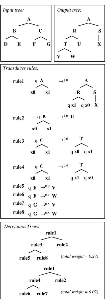
Figure 3: Derivation trees for an R tree transducer.
derivation trees forX automatically, we build a modified transducerX′. This new transducer produces derivation
trees on its output instead of normal output trees. X′ is
(Σ, R, Q, Qi, R′), with
R′≡ {(q, pattern, rule(yieldrhs(Q×paths)), w)|
rule= (q, pattern, rhs, w)∈R}
That is, the originalrhsof rules are flattened into a tree of depth 1, with the root labeled by the original rule, and all the non-expanding∆-labeled nodes of therhs re-moved, so that the remaining children are the nonterminal yield in left to right order. Derivation trees deterministi-cally produce a single weighted output tree.
The derived transducerX′ nicely produces derivation
trees for a given input, but in explaining an observed (input/output) pair, we must restrict the possibilities fur-ther. Because the transformations of an input subtree depend only on that subtree and its state, we can (Al-gorithm 1) build a compact wRTG that produces ex-actly the weighted derivation trees corresponding toX -transductions(I,()) ⇒∗
X (O, h) (with weight equal to
wX(h)).
6
Inside-Outside for wRTG
Given a wRTG G = (Σ, N, S, P), we can compute the sums of weights of trees derived using each produc-tion by adapting the well-known inside-outside algorithm for weighted context-free (string) grammars (Lari and Young, 1990).
The inside weights using G are given byβG : TΣ → (R−R−), giving the sum of weights of all tree-producing
derivatons from trees with nonterminal leaves:
βG(t)≡
X
(t,r,w)∈P
w·βG(r) ift∈N
Y
p∈pathst(N)
βG(labelt(p)) otherwise
By definition,βG(S)gives the sum of the weights of all trees generated byG. For the wRTG generated by DERIV(X, I, O), this is exactlyWX(I, O).
Outside weightsαGfor a nonterminal are the sums of weights of trees generated by the wRTG that have deriva-tions containing it, but excluding its inside weights (that is, the weights summed do not include the weights of rules used to expand an instance of it).
αG(n∈N)≡1ifn=S, else:
uses of n in productions
z X}| {
p,(n′,r,w)∈P:labelr(p)=n
w·αG(n′)·
Y
p′∈pathsr(N)−{p}
βG(labelr(p′))
| {z }
Algorithm 1: DERIV
Input: xR transducer X = (Σ,∆, Q, Qi, R) and ob-served tree pairI∈TΣ,O∈T∆.
Output: derivation wRTGG= (R, N ⊆Q×pathsI×
pathsO, S, P) generating all weighted deriva-tion trees forXthat produceOfromI. Returns
f alseinstead if there are no such trees. begin
S←(Qi,(),()),N ← ∅,P ← ∅ if PRODUCEI,O(S)then
return(R, N, S, P)
else
returnf alse
end
memoized PRODUCEI,O(q, i, o)returns boolean≡ begin
anyrule?←f alse
forr= (q, pattern, rhs, w)∈R:pattern(I↓i) = 1∧MATCHO,∆(rhs, o)do
(o1, . . . , on)←pathsrhs(Q×paths)sorted by
o1<lex . . . <lexon
//n= 0 if there are none
labelandrankderivrhs(())←(r, n) forj←1tondo
(q′, i′)←label
rhs(oj)
c←(q′, i·i′, o·o
i)
if¬PRODUCEI,O(c)then nextr
labelandrankderivrhs((j))←(c,0)
anyrule?←true
P←P∪ {((q, i, o), derivrhs, w)}
ifanyrule?thenN ←N∪ {(q, i, o)}
returnanyrule? end
MATCHt,Σ(t′, p)≡ ∀p′∈path(t′) :label(t′, p′)∈
Σ =⇒ labelandrankt′(p′) =labelandrankt(p·p′) The possible derivations for a given
PRODUCEI,O(q, i, o)are constant and need not be computed more than once, so the function is memoized. We have in the worst case to visit all|Q| · |I| · |O|
(q, i, o)pairs and have all|R|transducer rules match at each of them. If enumerating rules matching transducer input-patterns and output-subtrees has costL(constant given a transducer), then DERIV has time complexity
O(L· |Q| · |I| · |O| · |R|).
Finally, given inside and outside weights, the sum of weights of trees using a particular production is
γG((n, r, w)∈P)≡αG(n)·w·βG(r).
ComputingαG andβG for nonrecursive wRTG is a straightforward translation of the above recursive defi-nitions (using memoization to compute each result only once) and isO(|G|)in time and space.
7
EM Training
Estimation-Maximization training (Dempster, Laird, and Rubin, 1977) works on the principle that the corpus like-lihood can be maximized subject to some normalization constraint on the parameters by repeatedly (1) estimating the expectation of decisions taken for all possible ways of generating the training corpus given the current parame-ters, accumulating parameter counts, and (2) maximizing by assigning the counts to the parameters and renormal-izing. Each iteration is guaranteed to increase the like-lihood until a local maximum is reached.
Algorithm 2 implements EM xR training, repeatedly computing inside-outside weights (using fixed transducer derivation wRTGs for each input/output tree pair) to ef-ficiently sum each parameter contribution to likelihood over all derivations. Each EM iteration takes time linear in the size of the transducer and linear in the size of the derivation tree grammars for the training examples. The size of the derivation trees is at worstO(|Q|·|I|·|O|·|R|). For a corpus of K examples with average input/output sizeM, an iteration takes (at worst)O(|Q| · |R| ·K·M2) time—quadratic, like the forward-backward algorithm.
8
Tree-to-String Transducers (xRS)
We now turn to tree-to-string transducers (xRS). In the automata literature, these were first called generalized
syntax-directed translations (Aho and Ullman, 1971) and
used to specify compilers. Tree-to-string transducers have also been applied to machine translation (Yamada and Knight, 2001; Eisner, 2003).
We give an explicit tree-to-string transducer example in the next section. Formally, a weighted extended-lhs
root-to-frontier tree-to-string transducerXis a quintuple (Σ,∆, Q, Qi, R)whereΣis the input alphabet, and ∆ is the output alphabet, Qis a finite set of states, Qi ∈
Qis the initial (or start, or root) state, andR ⊆ Q×
XRP ATΣ×(∆∪(Q×paths))⋆×R+are a finite set of
weighted transformation rules, written(q, pattern)→w
rhs. A rule says that to transform (with weight w) an input subtree matchingpatternwhile in stateq, replace it by the string ofrhswith its nonterminal (Q×paths) letters replaced by their (recursive) transformation.
Algorithm 2: TRAIN
Input: xR transducerX = (Σ,∆, Q, Qd, R), observed weighted tree pairsT ∈TΣ×T∆×R+,
normal-ization functionZ({countr | r ∈ R}, r′ ∈ R), minimum relative log-likelihood change for con-vergenceǫ∈R+, maximum number of iterations
maxit ∈ N, and prior counts (for a so-called
Dirichlet prior){priorr |r∈R}for smoothing each rule.
Output: New rule weightsW ≡ {wr|r∈R}. begin
for(i, o, w)∈T do
di,o←
DERIV(X, i, o)//Alg. 1
ifdi,o=f alsethen
T ←T− {(i, o, w)}
warn(more rules are needed to explain (i,o))
compute inside/outside weights fordi,oand remove all useless nonterminalsnwhose
βdi,o(n) = 0orαdi,o(n) = 0
itno←0,lastL← −∞,δ←ǫ
forr= (q, pat, rhs, w)∈Rdowr←w whileδ≥ǫ∧itno < maxitdo
forr∈Rdocountr←priorr
L←0
for(i, o, wexample)∈T
//Estimate
do
letD≡di,o≡(R, N, S, P) computeαD, βDusing latest
W ≡ {wr|r∈R}
//see Section 6
forprod= (n, rhs, w)∈Pdo
γD(prod)←αD(n)·w·βD(rhs) letrule≡labelrhs(())
countrule←countrule+wexample·γDβD(prod(S))
L←L+ logβD(S)·wexample
forr= (q, pattern, rhs, w)∈R
//Maximize
do
wr←
countr
Z({countr|r∈R}, r) //e.g.Z((q, a, b, c))≡ X
r=(q,d,e,f)∈R
countr
δ← L−lastL |L|
lastL←L,itno←itno+ 1
end
are strings containing state-marked input subtrees). We have developed an xRS training procedure similar to the xR procedure, with extra computational expense to con-sider how different productions might map to different spans of the output string. Space limitations prohibit a detailed description; we refer the reader to a longer ver-sion of this paper (submitted). We note that this algo-rithm subsumes normal inside-outside training of PCFG on strings (Lari and Young, 1990), since we can always fix the input tree to some constant for all training exam-ples.
9
Example
It is possible to cast many current probabilistic natural language models as R-type tree transducers. In this sec-tion, we implement the translation model of (Yamada and Knight, 2001). Their generative model provides a formula for P(Japanese string|English tree), in terms of individual parameters, and their appendix gives spe-cial EM re-estimation formulae for maximizing the prod-uct of these conditional probabilities across the whole tree/string corpus.
We now build a trainable xRS tree-to-string transducer that embodies the same P(Japanese string|English tree). First, we need start productions like these, where q is the start state:
- q x:S→q.TOP.S x - q x:VP→q.TOP.VP x
These set up states like q.TOP.S, which means “translate this tree, whose root is S.” Then every q.parent.child pair gets its own set of three insert-function-word productions, e.g.:
- q.TOP.S x→i x, r x - q.TOP.S x→r x, i x - q.TOP.S x→r x - q.NP.NN x→i x, r x - q.NP.NN x→r x, i x - q.NP.NN x→r x
State i means “produce a Japanese function word out of thin air.” We include an i production for every Japanese word in the vocabulary, e.g.:
- i x→de - i x→kuruma - i x→wa
State r means “re-order my children and then recurse.” For internal nodes, we include a production for ev-ery parent/child-sequence and evev-ery permutation thereof, e.g.:
- r NP(x0:CD, x1:NN)→q.NP.CD x0, q.NP.NN x1 - r NP(x0:CD, x1:NN)→q.NP.NN x1, q.NP.CD x0 The rhs sends the child subtrees back to state q for re-cursive processing. However, for English leaf nodes, we instead transition to a different state t, so as to prohibit any subsequent Japanese function word insertion:
- r CC(x0:and)→t x0
State t means “translate this word,” and we have a produc-tion for every pair of co-occurring English and Japanese words:
- t car→kuruma - t car→wa - t car→*e*
This follows (Yamada and Knight, 2001) in also allowing English words to disappear, or translate to epsilon.
Every production in the xRS transducer has an associ-ated weight and corresponds to exactly one of the model parameters.
There are several benefits to this xRS formulation. First, it clarifies the model, in the same way that (Knight and Al-Onaizan, 1998; Kumar and Byrne, 2003) eluci-date other machine translation models in easily-grasped FST terms. Second, the model can be trained with generic, off-the-shelf tools—versus the alternative of working out model-specific re-estimation formulae and implementing custom training software. Third, we can easily extend the model in interesting ways. For exam-ple, we can add productions for multi-level and lexical re-ordering:
- r NP(x0:NP, PP(IN(of), x1:NP))→q x1, no, q x0 We can add productions for phrasal translations:
- r NP(JJ(big), NN(cars))→ooki, kuruma
This can now include crucial non-constituent phrasal translations:
- r S(NP(PRO(there),VP(VB(are), x0:NP)→q x0, ga, arimasu
We can also eliminate many epsilon word-translation rules in favor of more syntactically-controlled ones, e.g.:
- r NP(DT(the),x0:NN)→q x0
We can make many such changes without modifying the training procedure, as long as we stick to tree automata.
10
Related Work
Tree substitution grammars or TSG (Schabes, 1990) are equivalent to regular tree grammars. xR transduc-ers are similar to (weighted) Synchronous TSG, except that xR can copy input trees (and transform the copies differently), but does not model deleted input subtrees. (Eisner, 2003) discusses training for Synchronous TSG. Our training algorithm is a generalization of forward-backward EM training for finite-state (string) transducers, which is in turn a generalization of the original forward-backward algorithm for Hidden Markov Models.
11
Acknowledgments
Thanks to Daniel Gildea and Kenji Yamada for comments on a draft of this paper, and to David McAllester for help-ing us connect into previous work in automata theory.
References
Aho, A. V. and J. D. Ullman. 1971. Translations of a context-free grammar.
Information and Control, 19:439–475.
Alshawi, Hiyan, Srinivas Bangalore, and Shona Douglas. 2000. Learning de-pendency translation models as collections of finite state head transducers.
Computational Linguistics, 26(1):45–60.
Baker, J. K. 1979. Trainable grammars for speech recognition. In D. Klatt and J. Wolf, editors, Speech Communication Papers for the 97th Meeting of the
Acoustical Society of America. Boston, MA, pages 547–550.
Bangalore, Srinivas and Owen Rambow. 2000. Exploiting a probabilistic hierar-chical model for generation. In Proc. COLING.
Baum, L. E. and J. A. Eagon. 1967. An inequality with application to statistical estimation for probabilistic functions of Markov processes and to a model for ecology. Bulletin of the American Mathematicians Society, 73:360–363.
Charniak, Eugene. 2001. Immediate-head parsing for language models. In Proc.
ACL.
Chelba, C. and F. Jelinek. 2000. Structured language modeling. Computer Speech and Language, 14(4):283–332.
Collins, Michael. 1997. Three generative, lexicalised models for statistical pars-ing. In Proc. ACL.
Comon, H., M. Dauchet, R. Gilleron, F. Jacquemard, D. Lugiez, S. Tison, and M. Tommasi. 1997. Tree automata techniques and applications. Available on
www.grappa.univ-lille3.fr/tata. release October, 1st 2002.
Corston-Oliver, Simon, Michael Gamon, Eric K. Ringger, and Robert Moore. 2002. An overview of Amalgam, a machine-learned generation module. In
Proc. IWNLG.
Dempster, A. P., N. M. Laird, and D. B. Rubin. 1977. Maximum likelihood from incomplete data via the EM algorithm. Journal of the Royal Statistical Society,
Series B, 39(1):1–38.
Eisner, Jason. 2003. Learning non-isomorphic tree mappings for machine trans-lation. In Proc. ACL (companion volume).
Engelfriet, J. 1975. Bottom-up and top-down tree transformations—a compari-son. Math. Systems Theory, 9(3):198–231.
Gécseg, F. and M. Steinby. 1984. Tree Automata. Akadémiai Kiadó, Budapest. Gildea, Daniel. 2003. Loosely tree-based alignment for machine translation. In
Proc. ACL.
Joshi, A. and Y. Schabes. 1997. Tree-adjoining grammars. In G. Rozenberg and A. Salomaa, editors, Handbook of Formal Languages (Vol. 3). Springer, NY. Klein, Dan and Christopher D. Manning. 2003. Accurate unlexicalized parsing.
In Proc. ACL.
Knight, K. and Y. Al-Onaizan. 1998. Translation with finite-state devices. In
Proc. AMTA.
Knight, K. and D. Marcu. 2002. Summarization beyond sentence extraction— a probabilistic approach to sentence compression. Artificial Intelligence,
139(1).
Kumar, S. and W. Byrne. 2003. A weighted finite state transducer implemen-tation of the alignment template model for statistical machine translation. In
Proceedings of HLT-NAACL.
Langkilde, I. 2000. Forest-based statistical sentence generation. In Proc. NAACL.
Langkilde, I. and K. Knight. 1998. Generation that exploits corpus-based statisti-cal knowledge. In Proc. ACL.
Lari, K. and S. J. Young. 1990. The estimation of stochastic context-free gram-mars using the inside-outside algorithm. Computer Speech and Language, 4. Nederhof, Mark-Jan and Giorgio Satta. 2002. Parsing non-recursive CFGs. In
Proc. ACL.
Pang, Bo, Kevin Knight, and Daniel Marcu. 2003. Syntax-based alignment of multiple translations extracting paraphrases and generating new sentences. In
Proc. HLT/NAACL.
Rounds, William C. 1970. Mappings and grammars on trees. Mathematical
Systems Theory, 4(3):257–287.
Schabes, Yves. 1990. Mathematical and Computational Aspects of Lexicalized
Grammars. Ph.D. thesis, Department of Computer and Information Science,
University of Pennsylvania.
Thatcher, J. W. 1970. Generalized2sequential machine maps. J. Comput. System
Sci., 4:339–367.
Viterbi, A. 1967. Error bounds for convolutional codes and an asymptotically optimum decoding algorithm. IEEE Trans. Information Theory, IT-13. Wu, Dekai. 1997. Stochastic inversion transduction grammars and bilingual
pars-ing of parallel corpora. Computational Lpars-inguistics, 23(3):377–404.