Distributed representation and estimation of WFST-based n-gram models
Cyril Allauzen, Michael Riley and Brian Roark
Google, Inc.
{allauzen,riley,roark}@google.com
Abstract
We present methods for partitioning a weighted finite-state transducer (WFST) representation of an n-gram language model into multiple blocks orshards, each of which is a stand-alone WFST n-gram model in its own right, allowing process-ing with existprocess-ing algorithms. After in-dependent estimation, including normal-ization, smoothing and pruning on each shard, the shards can be reassembled into a single WFST that is identical to the model that would have resulted from estimation without sharding. We then present an ap-proach that uses data partitions in conjunc-tion with WFST sharding to estimate mod-els on orders-of-magnitude more data than would have otherwise been feasible with a single process. We present some num-bers on shard characteristics when large models are trained from a very large data set. Functionality to support distributed n-gram modeling has been added to the open-source OpenGrm library.
1 Introduction
Training n-gram language models on ever in-creasing amounts of text continues to yield large model improvements for tasks as diverse as ma-chine translation (MT), automatic speech recogni-tion (ASR) and mobile text entry. One approach to scaling n-gram model estimation to peta-byte scale data sources and beyond, is to distribute the storage, processing and serving of n-grams (Heafield, 2011). In some scenarios – most no-tably ASR – a very common approach is to heav-ily prune models trained on large resources, and then pre-compose the resulting model off-line with other models (e.g., a pronunciation lexicon) in or-der to optimize the model for use at time of first-pass decoding (Mohri et al., 2002). Among other
things, this approach can impact the choice of smoothing for the first-pass model (Chelba et al., 2010), and the resulting model is generally stored as a weighted finite-state transducer (WFST) in or-der to take advantage of known operations such as determinization, minimization and weight pushing (Allauzen et al., 2007; Allauzen et al., 2009; Al-lauzen and Riley, 2013). Even though the result-ing model in such scenarios is generally of mod-est size, there is a benefit to training on very large samples, since model pruning generally aims to minimize the KL divergence from the unpruned model (Stolcke, 1998).
Storing such a large n-gram model in a single WFST prior to model pruning is not feasible in many situations. For example, speech recognition first pass models may be trained as a mixture of models from many domains, each of which are trained on billions or tens of billions of sentences (Sak et al., 2013). Even with modest count thresh-olding, the size of such models before entropy-based pruning would be on the order of tens of billions of n-grams.
Storing this model in the WFST n-gram format of the OpenGrm library (Roark et al., 2012) allo-cates an arc for every n-gram (other than end-of-string n-grams) and a state for every n-gram prefix. Even using very efficient specialized n-gram rep-resentations (Sorensen and Allauzen, 2011), a sin-gle FST representing this model would require on the order of 400GB of storage, making it difficult to access and process on a single processor.
In this paper, we present methods for the dis-tributed representation and processing of large WFST-based n-gram language models by parti-tioning them into multiple blocks orshards. Our sharding approach meets two key desiderata: 1) each sub-model shard is a stand-alone “canonical format” WFST-based model in its own right, pro-viding correct probabilities for a particular subset of the grams from the full model; and 2) once n-gram counts have been sharded, downstream
ϵ
...
the
ϵ
ϵ the
end xyz
xyz ϵ end
ϵ
end
x
x
ϵ
<S> the
end <S>
end the
the
[image:2.595.88.274.64.204.2]xyz ...
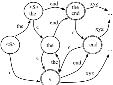
Figure 1: Schematic of canonical WFST n-gram format, unweighted for simplicity. Each state shows the history it encodes for convenience (they are actually unlabeled). Final states are denoted with double circle.
cessing such as model normalization, smoothing and pruning, can occur on each shard indepen-dently. Methods, utilities and convenience scripts have been added to the OpenGrm NGram library1
to permit distributed processing. In addition to presenting design principles and algorithms in this paper, we will also outline the relevant library functionality.
2 Canonical WFST n-gram format
We take as our starting point the standard ‘canon-ical’ WFST n-gram model format from Open-Grm, which is presented in Roark et al. (2012) and at ngram.opengrm.org, but which we summa-rize briefly here. Standard n-gram language mod-els can be presented in the following well-known backoff formulation:
P(w|h) =
ˆP(
w|h) ifc(hw)>0
α(h) P(w|h0) otherwise (1)
wherewis the word (or symbol) being predicted based on the previous history h, and h0 is the longest proper suffix of h (or if h is a single word/symbol). The backoff weightα(h)ensures that this is a proper probability distribution over symbols in the vocabulary, and is easily calculated based on the estimates ˆP for observed n-grams. Note that interpolated n-gram models also fit this formulation, if pre-interpolated.
Figure 1 presents a schematic of the WFST n-gram model format that we describe here. The WFST format represents n-gram histories h as states2, and wordsw following h as arcs leaving
1ngram.opengrm.org
2For convenience, we will refer to states as encoding (or representing) a historyh – or even just call the stateh – though there is no labeling of states, just arcs.
the state that encodesh. There is exactly one uni-gram state (labeled within Figure 1), which rep-resents the empty history. For every statehin the model other than the unigram state, there is a spe-cial backoff arc, labeled with, with destination state h0, the backoff state of h. For an n-gram hw, the arc labeled with w leaving history state hwill have as destination the state hwifhw is a proper prefix of another n-gram in the model; oth-erwise the destination will beh0w. The start state of the model WFST represents the start-of-string history (typically denoted<S>), and the end-of-string (</S>) probability is encoded in state final costs. Neither of these symbols labels any arcs in the model, hence they are not required to be part of the explicit vocabulary of the model. Costs in the model are generally represented as negative log counts or probabilities, and the backoff arc cost from statehis -logα(h).
With the exception of the start and unigram states, every state h in the model is the destina-tion state of an n-gram transidestina-tion originating from a prefix history, which we will term an ‘ascend-ing’ n-gram transition. If h = w1. . . wk is a
state in the model (k > 0 and if k = 1 then w1 6=<S>), then there also exists a state in the
model ¯h = w1. . . wk−1 and a transition from ¯h
to h labeled with wk. We will call a sequence
of such ascending n-gram transitions an ascend-ing path, and every state in the model (other than unigram and start) can be reached via a single as-cending path from either the unigram state or the start state. This plus the backoff arcs make the model fully connected.
3 Sharding count n-gram WFSTs
3.1 Model partitioning
sym-bols in the model to unique indices that label the arcs in the WFST. We use indices from this sym-bol table to define a total order<V on our
vocab-ulary augmented with start-of-string token which is assigned index 0.3 We then define the
colexi-cographic (or reverse lexicolexi-cographic) order<over V∗ recursively on the length of the sequences as follow. For allx, y6=, we have < xand
x < yiff
x|x|<V y|y|or,
x|x|=y|y|andx <¯ y¯ (2)
where x¯ denotes the longest prefix of x distinct fromxitself. The colexicographic interval[x, y)
then denotes the set of sequenceszsuch thatx ≤
z < y.
For example, assuming symbol indices the=1 and end=2, the colexicographic ordering of the states in Figure 1 is:
Colex. State histories Order (as words) (as indices)
0
1 <S> 0
2 the 1
3 <S>the 0 1
4 end 2
5 the end 1 2
If we want, say, 4 shards of this model (at least, the visible part in the schematic in Figure 1), we can partition the state histories in 4 intervals; for example:
{[,1),[1,2),[2,1 2),[1 2,3)}= {{,0},{1,0 1},{2},{1 2}}.
By convention, we write the interval [x, y) as x1. . . xl : y1. . . ym. Thus, the above partition
would be written as:4
0 : 1 1 : 2 2 : 1 2 1 2 : 3
While this partitions the states into subsets, it re-mains to turn these subsets into stand-alone, con-nected WFSTs with the correct topology to al-low for direct use of existing language model es-timation algorithms on each shard independently. For this to be the case, we need to: (1) be 3Not to be confused with the convention thathas index 0 in FST symbol tables.
4We omit the empty historyfrom the interval specifica-tion since it is always assigned to the first interval.
ϵ ϵ
ϵ the
xyz xyz
end
ϵ
end
x
x
ϵ
<S> the
end
end the
[image:3.595.332.499.67.198.2]xyz
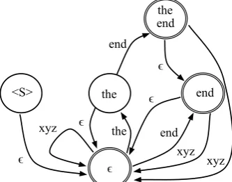
Figure 2: Schematic of a completed shard of the model in Figure 1. The state corresponding to the history ‘the end’ is the only state strictly in-context for this shard.
able to reach each state via the correct ascending path from the start or unigram state, with correct counts/probabilities; (2) have backoff states of all in-shard states, along with their arcs, for calculat-ing backoff costs; and (3) correctly assign all arc destinations within each new WFST.
3.2 Model completion
Given a set of states to include in a context shard, the shard model must be ‘completed’ to include all of the requisite states and arcs needed to con-form to the canonical n-gram topology. We step through each of the key requirements in turn. We refer to those states that fall within the context in-terval as ‘strictly in-context’. Figure 2 shows a schematic of the shard model that results for the context 1 2 : 3, which we will refer to when illustrating particular requirements. Only the state corresponding to ‘the end’ is strictly in-context for this particular shard. All states that are suffixes of strictly in-context states are also referred to as in-context (though notstrictly so), since they are needed for proper normalization – i.e., calculation ofα(h) in the recursive n-gram model definition in equation 1. Hence, the state corresponding to ‘end’ in Figure 2 is in-context and is included in the shard, as is the unigram state.
The start state and all states and transitions on ascending paths from the start and unigram states to in-context states must be included, so that states that are in-context can be reached from the start state. Thus, the state corresponding to ‘the’ in Fig-ure 2 must be included, along with its arc labeled with ‘end’, since they are on the ascending path to ‘the end’, which is strictly in-context.
destination must be the longest suffix of hw that has been included as a state in the shard model. The arcs labeled with ‘xyz’ in Figure 2 all point to the unigram state, since no states representing histories ending in ‘xyz’ are in the shard model.
For the small schematic example in Figures 1 and 2, there is not much savings from sharding af-ter completing the shard model: only one state and four arcs from the observed part of the model in Figure 1 were omitted in the schematic in Figure 2. And it is clear from the construction that there will be some redundancy between shards in the states and arcs included when the shard model is com-pleted. But for large models, each shard will be a small fraction of the total model. Note that there is a tradeoff between the number of shards and the amount of redundancy across shards.
Another way to view the shard model in Fig-ure 2 relative to the full model in FigFig-ure 1 is as a pruned model, where the arcs and states that were pruned are precisely those that are not needed within that particular shard. This perspective is useful when discussing distributed training in the next section.
4 Distributed training of n-gram models
When presenting model sharding in the previous section, we had access to the specific states in the model schematic, and defined the contexts accord-ingly. When training a model from data at the scale that requires distributed processing, the full model does not exist to inspect and partition. In-stead, we must derive the context sharding in some fashion prior to training the model. We will thus break this section into two parts: first, deriving context intervals for model sharding; then estimat-ing models given context intervals.
4.1 Deriving context intervals
Given a large corpus, there are a couple of ways to approach efficient calculation of effective con-text intervals. Effective in this case is balanced, i.e., one would like each sharded model to be of roughly the same size, so that the time for model estimation is roughly commensurate across shards and lagging shards are avoided.
The first approach is to build a smaller footprint model than the desired model, which would take a fraction of the time to train, then derive the con-texts from that model. For example, if one wanted to train a 5-gram model from a billion word cor-pus, then one may derive context intervals based
on trigram model trained by sampling one out of every hundred sentences from the corpus. Given that more compact model, it is relatively straight-forward to examine the storage required for each state and choose a balanced partition accordingly. At higher orders and with the full sample, the size of each shard may ultimately differ, but we have found that estimating relative shard sizes based on lower-order sampled models is effective at provid-ing functional context intervals. See section 5 for specific OpenGrm NGram library functionality re-lated to context interval estimation.
Another method for deriving context intervals is to accumulate the set of n-grams into a large collection, sort it by history in the same colexico-graphic order as is used to define the context in-tervals, and then take quantiles from that sorted collection. This can lead to more balanced shards than the previous method, though efficient meth-ods for distributed quantile extraction from collec-tions of that sort is beyond the scope of this paper.
4.2 Estimating models given context intervals
Given a definition ofkcontext intervalsC1. . . Ck,
we can train sharded models on very large data sets as follows:
1. Partition data intomdata shardsD1. . . Dm
2. For each data shardDi
(a) Count the n-grams from Di and build
full WFST n-gram representationTi
(b) SplitTiintokshard modelsTi1. . . Tik
3. For each context interval Cj, merge counts
T·jfrom all data shards: Fj = Mergemi=1(Tij)
4. Perform these global operations on collection F1. . . Fkto prepare for model estimation:
(a) Transfer correct counts as needed across shards (see Section 4.2.4 below). (b) Derive resources such as
count-of-counts by aggregating across shards. 5. Normalize, smooth, prune eachFjas needed:
Mj= MakeModel(Fj)
6. Merge model shards:M= Mergek
j=1(Mj)
We now go through each of these 6 stages one by one in the following sub-sections.
4.2.1 Partition data
4.2.2 Count and split data shards
For each data shardDi, perform n-gram counting
exactly as one would in a non-distributed scenario. (See Section 5 for specific commands within the OpenGrm NGram library.) This results in an n-gram count WFST Ti for each data shard.
Us-ing the context interval specifications C1. . . Ck
we then splitTiintokshard models. Because we
have the full modelTi, we can determine exactly
which states and arcs need to be preserved for each context interval, and prune the rest away.
4.2.3 Merge sharded models
For each context intervalCj, there will be a shard
model Tij for every data shard Di. Standard
count merging will yield the correct counts for all in-context n-grams and the correct overall model topology, i.e., every state and arc that is required will be there. However, n-grams that are not in-context may not have the correct count, since they may have occurred in a data shard but were not in-cluded in the context shard due to the absence of any in-context n-grams for which it is a prefix.
To illustrate this point, consider a scenario with just two data shards, D1 and D2, and a context
shardCjthat only includes the n-gram history ‘foo
bar baz’ strictly in-context. Suppose ‘foo bar’ oc-curs 10 times inD1and also 10 times inD2, while
‘foo bar baz’ occurs 3 times inD1 but doesn’t
oc-cur at all inD2. Recall that states and ascending
arcs that are not in-context are only included in the shard model as required to ascend to the in-context states. In the absence of ‘foo bar baz’ in T2j, the n-gram arc and state corresponding to ‘foo
bar’ will not be included in that shard, despite hav-ing occurred 10 times inD2. When the counts in
T1jandT2jare merged, ‘foo bar’ will be included
in the merger, but will only have counts coming fromT1j. Hence, rather than the correct count of
20, that n-gram will just have a count of 10. The correct count of ‘foo bar’ is only guaranteed to be found in the shard for which it is in-context.
To get the correct counts in every shard that needs them, we must perform a transfer opera-tion to pass correct counts from shards where n-grams are strictly in-context to shards where they are needed as prefixes of other n-grams.
4.2.4 Global operations on the collection
Transfer: As mentioned above, count merging of
sharded count WFSTs across data shards yields correct counts for in-context states, as well as the correct WFST topology – i.e., all needed n-grams
are included – but is not guaranteed to have the correct counts of n-grams that are not in-context. For each shard Fi, however, we know which
n-grams we need to get the correct count for, and can easily calculate the context shard that these n-grams fall into. Using that information, a transfer of correct counts is effected via the following three stages:
1. For each shardFi, for eachFj (j6=i), prune
Fi to only those n-grams that are strictly
in-context for in-contextCj, and send the resulting
Fij to shardFj to give correct counts.
2. For every shardFj, provide correct counts for
each incomingF·j requiring them and return
to the appropriate shardFi.
3. For every shard Fi, update counts from
in-comingFi·.
Only needed n-grams are processed in this trans-fer algorithm, which we will term the “standard” transfer algorithm in the experimental results. Let Qi be the set of states for shard Fi. Each state
is an n-gram of length less than n (where n is the order of the model) that must have its cor-rect count requested from the shard where it is strictly in context. This leads to a complexity of O(nPki=1|Qi|).
state that is strictly in-context. The latter condi-tion holds if the n-gram arc’s origin state is out-of-context, its destination state is in-context (though not strictly in-context), and the n-gram is not a pre-fix of any in-context state. We will call an n-gram of order n that meets either of those conditions “needed at ordern”. Then, for each ordernfrom 1 to the highest order in the model, transfer is car-ried out by replacing step number 1 in the standard transfer algorithm above with the following:
1. For each shardFi, for eachFj (j6=i), prune
Fi to only those n-grams that are strictly
in-context for in-contextCj, and are needed at
or-dern, along with all prefixes of such n-grams. If the resulting Fij is non-empty, send it to
shardFjto give correct counts.
The rest of transfer at order n proceeds as be-fore. In this algorithm, a shard requests an n-gram only if the destination state of its corresponding n-gram arc is in-context. This leads to a complex-ity inO(nPki=1|Qc
i|)whereQci denotes the set of
states in shardFicorresponding to in-context
his-tories for that shard. This is a complexity reduc-tion from the standard transfer algorithm above, since|Qi|/n <|Qci|<|Qi|.
Counts-of-counts: Deriving counts-of-count
his-tograms is key for certain smoothing methods such as Katz (1987). Each shard Fi can
pro-duce a histogram from only those n-grams that are strictly in-context, then the histograms can be aggregated straightforwardly across shards to produce a global histogram, since each n-gram is strictly in-context in only one shard.
4.2.5 Process count shards
Given the correct counts in each of the count shards Fi, we can proceed to use existing,
stan-dard n-gram processing algorithms to normalize, smooth and prune each of the models indepen-dently. These algorithms are linear in the size of the model being processed. With some minor exceptions, existing WFST-based language mod-eling algorithms, such as those in the OpenGrm NGram library, can be applied to each shard in-dependently. We mention two such exceptions in turn, both impacting the correct application of model pruning algorithms after the model shard has been normalized and smoothed.
First, whereas common smoothing algorithms such as Katz (1987) and absolute discounting (Ney et al., 1994) will properly discount and nor-malize all n-grams in the model shard, Witten-Bell smoothing (Witten and Witten-Bell, 1991) will yield
correct smoothed probabilities for icontext n-grams, but for n-grams not in-context in the cur-rent shard, the smoothed probabilities will not be guaranteed to be correctly estimated. This is be-cause Witten-Bell smoothing is defined in terms of the number of words that have been observed following a particular history, which in the WFST encoding of the n-gram model is represented by the number of arcs (other than the backoff arc) leaving the history state (plus one if the state is final). While for any in-context stateh, all of the arcs leaving the state will be present, some of the other n-gram states that were included to create the model topology – notably the states along the ascending path to in-context states – will not typ-ically have all of the arcs that they have in their own shard. Hence the denominator in Witten-Bell smoothing (the count of the state plus the number of words observed following the history) cannot be calculated locally, and the direct application of the algorithm will end up with mis-estimated n-gram probabilities along the ascending paths.
If no pruning is done, then only the in-context probabilities matter, and merging can take place with no issues (see the next section 4.2.6).
Pruning algorithms, however, such as relative entropy pruning (Stolcke, 1998), typically use the joint n-gram probability – P(hw) – when calcu-lating the scores that are used to decide whether to prune the n-gram or not. This joint probability is calculated by taking the product of all ing path conditional probabilities. If the ascend-ing path probabilities are wrong, these scores will also be wrong, and pruning will proceed in error. For Katz and absolute discounting, the ascend-ing probabilities are correct when calculated on the shard independently of the other shards (when given counts-of-counts); but Witten Bell will not be immediately ready for pruning.
To get correct pruning for a sharded Witten-Bell model, another round of the transfer algo-rithm outlined in Section 4.2.4 is required, to re-trieve the correct probabilities of ascending arcs in each shard.
cal-culated for every n-gram in the collection and then these scores sorted to derive the right threshold. This requires a process not unlike the counts-of-counts aggregation presented in Section 4.2.4, yet with a sorting of the collection rather than compi-lation into a histogram.
Once all of the model shards have been normal-ized, smoothed and pruned using standard WFST-based n-gram algorithms, the shards can be re-assembled to produce a single WFST.
4.2.6 Merge model shards
Merging the shard models into a single WFST n-gram model is a straightforward special case of general model merging, whereby two models are merged into one. In general, model merging al-gorithms of two WFST models with canonical n-gram topology will: (a) result in a new model with canonical n-gram topology; and (b) the n-gram costs in the new model are some function of the n-gram costs in the two models. If the models are being linearly interpolated, then the n-gram proba-bility will be calculated asλp1+ (1−λ)p2, where
pkcomes from thekth model, and the n-gram cost
will be the negative log of that probability.5
To merge model shards M1 and M2, we must
know, for each stateh, whetherhis in-context for M1orM2. The n-gram cost in the merged model
isc2 ifh is in-context forM2; andc1 otherwise,
whereck is the cost of the n-gram inMk. If we
start with an arbitrary model shard and designate that as M1, then we can merge each other shard
into the merged model in turn, and designate the resulting merged model as M1 for a subsequent
merge. By the end of merging in every context, all of the n-grams in the final model will have been merged in, so they will all have received their cor-rect probabilities. The resulting WFST will have the same probabilities as it would if the model had been trained in a single process.
5 OpenGrm distributed functionality
While most of these distributed functions will likely be implemented in some kind of large, data-parallel processing system6, such as MapReduce
(Dean and Ghemawat, 2008), these pipelines will rely upon core OpenGrm NGram library functions to count, make, prune and merge models. The 5Backoff arc costs can then be calculated in closed form. 6We have implemented an end-to-end pipeline, which makes use of the OpenGrm NGram library, in Flume (Cham-bers et al., 2010). Results in Section 6 were generated with this pipeline.
OpenGrm NGram library now includes some dis-tributed functionality, along with a convenience script to illustrate the sort of approach we have de-scribed in this paper.
Recall that the basic approach involves shard-ing the data, countshard-ing n-grams on each data shard separately, and then splitting the counts from each data shard into context shards. Two command-line utilities in OpenGrm provide functionality for (1) defining context shards; and (2) splitting an n-gram WFST based on given context shards. One method described in Section 4.1 for deriving con-text shards is to train a smaller model (e.g., lower order and/or sampled from the full target training scenario) and then derive balanced context shards from that smaller model. For example, if we want to train a 5-gram model on 1B words of text, we might count7trigrams from every 100th sentence,
yielding the n-gram count WFST 3g.fst. Then the command line binaryngramcontextcan make use of the sampled counts to derive a balanced sharding of the requested size:
ngramcontext --contexts=10 3g.fst >ctx.txt The resulting text file (ctx.txt) will look something like this:
0 : 18 18 : 307 35 307 35 : 70
70 : 147 ...
as discussed in Section 3.1. Given these con-text definitions, we can now use ngramsplit to partition full count WFSTs derived from partic-ular data shards. For example, suppose that we counted 5-grams from data shard k, yielding DS-k.5g-counts.fst. Then we can produce 10 count shards as follows:
ngramsplit --contexts=ctx.txt --complete \ DS-k.5g-counts.fst DS-k.5g-counts
which would result in 10 count shard WFSTs DS-k.5g-counts.0000i for 0 ≤ i < 10. The --complete flag ensures that all required n-grams are included in the shard, not just those strictly in-context. Once this has been done for all data shards, the counts for each context shard can be merged across the data shards, i.e., ngrammerge using the count merge method on DS-*.5g-counts.0000ifor alli.
n-grams time (hours) to pct. in- largest to
Corpus target preproc. make, model context smallest
(words; sents) order total per shard + count prune + shards ngrams shard ratio
Billion word 3 238M 4M 1.5 1.2 59 56.0 1.20
benchmark (BWB) 40M 1.6 1.6 5 84.8 1.07
(769M; 30.3M) 5 1.14B 4M 4.1 2.0 285 36.8 2.07
40M 4.7 3.5 28 50.5 1.26
Search queries (SQ) 5 16.6B 4M 23.4 8.9 5090 38.8 1.93
[image:8.595.75.525.61.183.2](70B; 13.2B) 40M 10.2 7.1 502 64.4 1.77
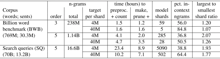
Table 1:Sharding characteristics and time to estimate under different training scenarios. As noted in Section 6, times are not comparable if n-gram order or size of corpus are different, and times should be interpreted as a relatively coarse measure of work. The last two columns (100*in-context/total n-ngrams and the ratio of sizes in ngrams) indicate shard redundancy. splitting again and using the command line binary
ngramtransfertwice: once to extract the correct counts from the correct shards; and once to return the extracted counts to the shards requesting them. We refer the reader to Section 4.2.4 for high level detail, and the convenience scriptngram.shin the OpenGrm NGram library for specifics.
Several new functions have been added via options to existing command line binaries in the OpenGrm NGram library. For example, ngramcount can now produce counts of counts (--method=count of counts) and produce them only for a specified context shard. Further, ngrammergehas acontext mergemethod, which uses a derived class of OpenGrm’s NGramMerge class to correctly reassemble count or language model sharded WFSTs into a single WFST. See the script ngram.sh in the OpenGrm NGram li-brary for details.
In the next section, we provide some data on the characteristics of n-gram models of different orders and sizes when they are trained via shard-ing.
6 Shard size versus redundancy
As stated earlier, we use Flume (Chambers et al., 2010) in C++ to distribute our OpenGrm NGram model training. This system is not currently pub-licly available, but within it we use methods gen-erally very similar to what is available in Open-Grm, just pipelined together in a different way. One difference between the Flume version and ngram.sh is the method for deriving contexts, which in Flume is based on efficient quantiles ex-tracted from the set of n-grams. While this is also a sampling method for deriving the contexts, the ordering constraints of quantiles do often lead to better (though not perfect) estimates of bal-anced shards. Additionally, the Flume system that was used to generate these numbers uses a smart
distributed processing framework, which allocates processors based on estimated size of the process. This impacts the interpretability of timing results, as noted below.
Table 1 presents some characteristics of lan-guage model training under several conditions which demonstrate some of the tradeoffs in dis-tributing the model in slightly different ways. From the Billion Word Benchmark (BWB) cor-pus (Chelba et al., 2014), we train trigram and 5-gram language models with different parameteri-zations for determining the model sharding. We also report results on a proprietary 70 billion word collection of search queries (SQ), also with differ-ent sharding parameterizations. For the BWB tri-als, no symbol or n-gram frequency cutoffs were used, but for the search queries, as part of the pre-processing and counting, we selected the 4 mil-lion most common words from the collection to include in the vocabulary (all others mapped to an out-of-vocabulary token) and limited 4-grams and 5-grams to those occurring at least twice or 4 times, respectively. All trigram models were pruned to 50 million n-grams prior to shard merg-ing (reassemblmerg-ing into a smerg-ingle WFST), and 5-gram models were pruned to 100 million n-5-grams. For these trials, the standard transfer algorithm in Section 4.2.4 was used. Run times are averaged over five independent runs.
target trans. time (hours) to count per by before trans. Task shard order trans. to end total
BWB 4M N 2.4 1.7 4.1
Y 2.1 3.5 5.5
40M N 2.6 2.1 4.7
Y 3.1 5.9 9.0
SQ 4M N 4.7 18.7 23.4
Y 4.5 7.6 12.1
40M N 5.7 4.4 10.2
[image:9.595.72.288.62.211.2]Y 5.9 6.7 12.6
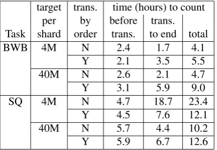
Table 2:Counting time broken down between stages occur-ring before transfer and those occuroccur-ring from transfer to the end of counting, using either the original transfer algorithm or transferring by order.
prune, etc. times). With larger shard sizes (and hence fewer shards), the percentage of n-grams in each shard that are in-context (rather than ascend-ing or backoff n-grams) is higher, and the size of the largest shard (in terms of total n-grams in the shard, both in-context and not) is much closer in size to the smallest shard, leading to better load balancing. Smaller shards, however, will gener-ally distribute more effectively for many of the es-timation tasks, leading to some speedups relative to fewer, larger shards.
Table 2 presents counting times for the 5-gram trials using both the standard transfer algorithm reported in Table 1 and the alternate “by order” transfer algorithm outlined in Section 4.2.4. The times are broken down into the part of counting before transfer and the part including transfer un-til the end. From these we can see that in scenar-ios with a very large number of shards – e.g., SQ with 4M target per shard, which yields more than 5000 shards – the “by order” transfer algorithm is much faster than the standard algorithm, leading to a factor of 2 speedup overall. However, increas-ing the target number of n-grams per shard, thus yielding fewer shards, is overall a more effective way to speedup processing. For much larger train-ing scenarios, when even 40M n-grams per shard would yield a large number of shards, one would expect this alternative transfer algorithm to be use-ful. Otherwise, the additional overhead of the ad-ditional stages simply adds to the processing time.
7 Related work
Brants et al. (2007) presented work on distributed language model training that has been very influ-ential. In that work, n-grams were sharded based
on a hash function of the first words of the n-gram, so that prefix n-grams, which carry normalization counts, end up in the same shard as those requir-ing the normalization. Because suffix n-grams do not end up in the same shard, smoothing methods that need access to backoff histories, such as Katz, require additional processing.
In contrast, our sharding is on the suffix of the history, which ensures that all n-grams with the same history fall together, and very often the backoff histories also fall in the same shard with-out having to be added. Since normalization val-ues can be derived by summing the counts of all n-grams with the same history, the prefix is not strictly speaking required for normalization, though, as described in Section 3.2, we do add them when ‘completing’ a model shard to canoni-cal WFST n-gram format.
Sharding with individual n-grams as the unit rather than working with the more complex WFST topologies does have its benefits, particularly when it comes to relatively easy balancing of shards. The primary benefit of using WFSTs in such a distributed setting lies in making use of WFST functionality, such as modeling with expected frequencies derived from word lattices (Kuznetsov et al., 2016). Additionally, sharding on the suffix of the history does allow for scaling to much longer n-gram histories, such as would arise in character language modeling. If we train a 15-gram character language model from stan-dard English corpora, then a significant number of those n-grams will begin with the space charac-ter, so creating a shard from a two character pre-fix may lead to extremely unbalanced sharding. In contrast, intervals of histories allow for balance even in such an extreme setting.
8 Summary and Future Directions
References
Cyril Allauzen and Michael Riley. 2013. Pre-initialized composition for large-vocabulary speech recognition. InProceedings of Interspeech, pages 666–670.
Cyril Allauzen, Michael Riley, Johan Schalkwyk, Wo-jciech Skut, and Mehryar Mohri. 2007. OpenFst: A general and efficient weighted finite-state transducer library. InImplementation and Application of Au-tomata, pages 11–23. Springer.
Cyril Allauzen, Michael Riley, and Johan Schalkwyk. 2009. A generalized composition algorithm for weighted finite-state transducers. InProceedings of Interspeech, pages 1203–1206.
Thorsten Brants, Ashok C Popat, Peng Xu, Franz J Och, and Jeffrey Dean. 2007. Large language mod-els in machine translation. In Proceedings of the Joint Conference on Empirical Methods in Natural Language Processing (EMNLP) and Computational Natural Language Learning (CoNLL).
Craig Chambers, Ashish Raniwala, Frances Perry, Stephen Adams, Robert R Henry, Robert Bradshaw, and Nathan Weizenbaum. 2010. Flumejava: easy, efficient data-parallel pipelines. In ACM Sigplan Notices, volume 45-6, pages 363–375.
Ciprian Chelba, Thorsten Brants, Will Neveitt, and Peng Xu. 2010. Study on interaction between en-tropy pruning and Kneser-Ney smoothing. In Pro-ceedings of Interspeech, pages 2422–2425.
Ciprian Chelba, Tomas Mikolov, Mike Schuster, Qi Ge, Thorsten Brants, Phillipp Koehn, and Tony Robin-son. 2014. One billion word benchmark for mea-suring progress in statistical language modeling. In Proceedings of Interspeech, pages 2635–2639. Jeffrey Dean and Sanjay Ghemawat. 2008.
Mapre-duce: simplified data processing on large clusters. Communications of the ACM, 51(1):107–113. Kenneth Heafield. 2011. Kenlm: Faster and smaller
language model queries. InProceedings of the Sixth Workshop on Statistical Machine Translation, pages 187–197. Association for Computational Linguis-tics.
Slava M. Katz. 1987. Estimation of probabilities from sparse data for the language model component of a speech recognizer. IEEE Transactions on Acoustics, Speech and Signal Processing, 35(3):400–401. Vitaly Kuznetsov, Hank Liao, Mehryar Mohri, Michael
Riley, and Brian Roark. 2016. Learning n-gram lan-guage models from uncertain data. InProceedings of Interspeech (to appear).
Mehryar Mohri, Fernando Pereira, and Michael Ri-ley. 2002. Weighted finite-state transducers in speech recognition. Computer Speech & Language, 16(1):69–88.
Hermann Ney, Ute Essen, and Reinhard Kneser. 1994. On structuring probabilistic dependences in stochas-tic language modeling. Computer Speech and Lan-guage, 8:1–38.
Brian Roark, Richard Sproat, Cyril Allauzen, Michael Riley, Jeffrey Sorensen, and Terry Tai. 2012. The OpenGrm open-source finite-state grammar soft-ware libraries. InProceedings of the ACL 2012 Sys-tem Demonstrations, pages 61–66.
Hasim Sak, Yun-hsuan Sung, Franc¸oise Beaufays, and Cyril Allauzen. 2013. Written-domain language modeling for automatic speech recognition. In Pro-ceedings of Interspeech, pages 675–679.
Jeffrey Sorensen and Cyril Allauzen. 2011. Unary data structures for language models. InProceedings of Interspeech, pages 1425–1428.
Andreas Stolcke. 1998. Entropy-based pruning of backoff language models. In Proceedings of the DARPA Broadcast News Transcription and Under-standing Workshop, pages 270–274.