Master thesis
Implementing and simulating the cross-entropy
ant system
Jonathan Brugge
Contents
Preface vii
Introduction and contributions ix
I
The Cross Entropy Ant System
1
1 Background 3
2 The Cross Entropy Ant System 5
2.1 Foraging ants . . . 5
2.2 CEAS . . . 6
2.2.1 Introduction . . . 6
2.2.2 Implementation . . . 7
2.2.3 Avoiding converging to a local optimum . . . 7
2.2.4 Cycles in paths . . . 8
2.2.5 Extensions . . . 8
II
Porting CEAS to ns-3
11
4 About ns-3 15
4.1 Introduction . . . 15
4.2 Features . . . 16
5 CEAS in ns-3 - the architecture 19 5.1 Overview . . . 19
5.2 Temperature table . . . 20
5.3 Pheromone table . . . 20
5.4 Ant packets . . . 21
5.4.1 Neighbour discovery packets . . . 24
5.5 Routing protocol . . . 25
5.5.1 Before sending the ants . . . 25
5.5.2 Leaving nodeA. . . 25
5.5.3 Passing through nodeB . . . 26
5.5.4 Arriving at nodeC . . . 27
5.5.5 The way back . . . 27
5.6 Infrastructure . . . 27
6 Validation 29 7 Experience with ns-3 33 7.1 Comparison with ns-2 . . . 34
7.1.1 Abstraction level . . . 34
7.1.2 Usability and adaptability . . . 35
7.1.3 Built-in components and models . . . 36
7.1.4 Experiment setup, control and analysis . . . 36
7.1.6 Efficiency . . . 37
III
Simulation and optimization
39
8 Simulation 41 8.1 Introduction . . . 418.2 The scenario . . . 41
8.2.1 The layout . . . 41
8.3 Basic results . . . 43
8.4 Load-sensitive cost functions . . . 45
8.5 Preplanning . . . 51
8.6 Packet format improvements . . . 51
9 Conclusion 55 9.1 The original plan . . . 55
9.2 What actually happened . . . 55
9.3 Future work . . . 57
A Simulation parameters 59
B Paper 61
C Presentation TM8105 69
Preface
This report describes the work I have done as my graduation project at NTNU in Trondheim. The work was performed within the Telematics department of the university under supervision of Poul Heegaard and Laurent Paquereau. At my home university in Enschede, Pieter-Tjerk de Boer was my first supervisor, with Geert Heijenk taking the role of second supervisor.
I would like to thank them for their help with this project. Pieter-Tjerk always spots the even smallest issues, whether they are mistakes in some formula in the research project or layout problems deeply hidden in the bibliography. I enjoyed the mix of discussing those issues and discussing everything else - from university politics to bicycle holidays. Thanks for that!
In Norway, Poul and Laurent took over - and kept doing that, even when results took longer than expected to arrive and graphs managed to deviate from the expected results in a surprising number of different ways. Extra meetings to find the last bugs and an Easter holiday spent writing a paper with Laurent -my project definitely took more of your time than the standard NTNU thesis. Thanks for all your help along the way!
Jonathan Brugge
Introduction and
contributions
For this thesis project, I have worked on the Cross-Entropy Ant System (CEAS), a routing protocol developed at NTNU. CEAS had been implemented in network simulator ns-2 [1]. At the start of the project, the plan was to
• Implement CEAS in ns-3
• Verify the implementation against the existing ns-2 implementation
• Come up with improvements to CEAS for use in environments with a relatively high rate of changes in the network topology
• Simulate the improvements to verify them
Ns-3 is a new simulator, written by the developers of ns-2, but otherwise incom-patible.
During the project, it became clear that porting to ns-3 was more work than originally expected. Thus, a relatively big part of this report is dedicated to the work done to implement CEAS in ns-3. The last part is about the additional scenarios that have been simulated with the ns-3 implementation and the specific improvements that have been made.
Where applicable, parameters used for the simulation have been included in this report. An earlier study [2] found that many studies in the field of network simulation lack information about the parameters, making it difficult to verify the results. The source code used for all simulations is available on request.
Structure
This thesis starts with an introduction to CEAS, including existing extensions to the system. It is followed by an introduction to ns-3 in chapter 3 and 4. Chapter 5 describes how CEAS has been implemented and how it fits in ns-3. The implementation is then validated against the existing ns-2 implementation in chapter 6. Some remarks about ns-3, derived from the experience of imple-menting CEAS in it, form chapter 7.
Improvements to CEAS to make it more usable in congested networks are dis-cussed in chapter 8, which also includes simulations of such networks. Conclu-sions follow in chapter 9, after which some appendices are included.
Contributions
The original goal of the project was to improve CEAS by making it more suit-able for highly dynamic networks. Others have worked on different projects to improve CEAS: the most important examples are the addition of a system called elite selection, described in [3], and the subpath extension, introduced in [4]. Both extensions are described in section 2.2.5 of this report.
Part I
Chapter 1
Background
Requirements to networks are changing over time and with those, the require-ments to routing protocols. New developrequire-ments mean that it is not necessarily enough to find a single shortest route from a source to a destination, but that specific requirements are placed on the quality of service offered by different paths and the possibility to balance the load between paths.
Different approaches are used to develop new routing protocols that fulfill those requirements. One approach is the use of algorithms inspired by the behaviour of swarms of animals, specifically ants [5]. A protocol based on how ants find their way to food was proposed in [6].
One example of an ant-based routing system, designed with the new require-ments in mind, is the Cross Entropy Ant System (CEAS). Cross-Entropy Ant System (CEAS) is a fully decentralized Ant Colony Optimization (ACO) sys-tem [7] first introduced in [8] and developed at NTNU. Different from some other systems, it uses the cross-entropy method as a mathematical basis.
This thesis does not contain an in-depth description of the cross-entropy method: it has been described in the research project, which was written as a preparation for this thesis project and is attached to this report as appendix D. An extensive introduction to the cross-entropy method can be found in [9].
Chapter 2
The Cross Entropy Ant
System
The Cross Entropy Ant System (CEAS) is a routing protocol developed at NTNU that takes ideas from nature, specifically how foraging ants find their way, to build an efficient and robust routing protocol. A basic description can be found in [11]. It is an example of a swarm-based routing protocol. CEAS uses the cross entropy method to quickly converge to good routes.
Note that the following is not a complete description of CEAS: it is intended to provide the information needed to understand the rest of this thesis. More information about CEAS cna be found in [11] and its references.
2.1
Foraging ants
CEAS takes its basic idea from nature. Consider an area with an ant nest and a place with food, respectively called “s” and “d” for “source” and “destination”. Each individual ant tries to find a way from the source to the destination. While travelling, it leaves a trail of pheromones. Those pheromones evaporate over time. Thus, if an ant uses a short route, it will pass there more often per unit of time on its way from the source to the destination and back again, resulting in a high concentration of pheromones on that route.
not communicate directly with each other, yet specific behaviour for the whole group emerges, is called emergent behaviour.
2.2
CEAS
2.2.1
Introduction
A number of routing protocols, such as AntHocNet, are designed after the for-aging ant behaviour described before. CEAS does that as well, but - contrary to the other protocols - bases it on the cross entropy method, which provides a mathematical basis for CEAS. The basic method is described in [12], though it is not directly applied to CEAS there. An overview of the algorithms used in CEAS can be found in [11].
The basic routing information in the protocol is a value pt,r,s, which is the
routing probability that a packet will go to node s, when it is at node r at iterationt. For all nodes, these probabilities can be grouped in a matrixpt= pt,rs∀rs. The routing probabilities are the ’digital pheromones’ of the protocol:
the higher the pheromone value from r to s, the higher the probability that a packet will travel over that link as its next hop.
The protocol also uses atemperature γt, which converges to a value based on the
cost of the best (lowest cost) route between two nodes. A performance function h(p, γ) indicates how good a certain matrixpis.
The algorithm works as follows:
1. Start with a set of routing probabilities pt=0 that are for instance uni-formly distributed: all paths have the same probability 1/n with n = size(s).
2. Generate a number of sample paths and select those samples that give the best results - so find a γ as low as possible, that still gives a certain number of cases that satisfyh(p, γ).
3. Using those samples, generate a new matrix pt which is as similar as possible to the optimal matrix. This optimal matrix is a matrix such that routes generated with it are the shortest routes, i.e. the matrix which, when used, results in the lowest possible temperature γ.
4. Increasetby 1 and repeat the procedure with the new matrix. Stop when the temperatureγ stabilizes.
Fort→ ∞, pt gets an optimal solution, wherept→∞,r,s is either 1 (if the link
performance function used in CEAS is h(p, γt) = e− Lt
γt, with Lt the cost at
timet. A more in-depth description can be found in section 2.3 in [3].
This procedure needs a number of samples before it can update the temperature and the matrix, which is not practical in a routing environment: it would be better if the probabilities would be updated with each arriving routing packet, instead of waiting for a batch of packets to arrive. CEAS achieves that by adjusting the performance function every time new information arrives, basing it on both the new information and the currently used function.
2.2.2
Implementation
To implement the behaviour described above, the routing protocol uses packets calledants. Ants travel from a source to a destination, possible using the matrix
pt to choose the route, accumulating the cost of the followed path. At the destination, the temperature is updated. The ant then travels back along the same way to the source, updatingptin the nodes it passes.
2.2.3
Avoiding converging to a local optimum
With the algorithm described above, there is a risk of ending up with a path that is not actually the shortest. At first, a reasonable - but not optimal - path pR may be found. No other paths have any pheromone at all, so all ants choose
to followpR. No better path is ever found.
To avoid that situation, CEAS knows two different kind of ants. Normal forward ants use the pheromone tables to find their destination, while explorer ants simply pick a random next hop, not using the pheromone values at all. Using a suitable mix of normal ants and explorer ants results in new routes being found, while known routes are reinforced with the right amount of pheromone.
That does not solve the whole problem, however. Consider the situation where the reasonable pathpR is known. At some point, a shorter route pB is found.
However, the chance of taking that route is not very high, as only one (explorer) ant ’deposited’ pheromone on that route, compared to possibly thousands of ants onpR. Thus, pB is not chosen more often and its pheromone value is not
reinforced.
2.2.4
Cycles in paths
Given how ants find their way to a destination, it is possible that an ant visits a single node twice on its way to the destination. In that case, the path to the destination will contain a cycle. In most cases, such cycles are not a problem as the system will converge to a route without cycles: a route with cycles can not be the best route to a destination, assuming a positive cost for every hop in the path.
In some cases, cycles can be a problem. Updating paths which contain a cycle means that ants have to travel more, resulting in a higher network load. Also, investing ’energy’ in longer paths might cause a longer time to converge to the shortest path. For some possible extensions to CEAS, such as subpaths (dis-cussed in 2.2.5), the effects can be noticable. In [13], three different approaches to handling cycles in CEAS are discussed. For the simulations in this report, cycles are detected at every hop and packets are dropped if they contain a cycle.
To avoid the creation of cycles, an extra mechanism has been used. Before the next hop of an ant is chosen, all nodes that it has visited before are taken out of the list of possible options. Though this heuristic has limitations in the current ns-3 implementation of CEAS, it prevents the most common cases, such as ants travelling back to the node from which they just came.
2.2.5
Extensions
The system described above works, but it is not as efficient as it could be. A number of improvements are already known that speed up convergence or reduce the overhead of the protocol by limiting the number of ant transmissions needed to get good routes.
Elite selection is one such optimization. When a forward ant reaches its des-tination, it is only converted to a backward ant if the cost for the path it has followed is within a certain distance from the best path known to that destina-tion. Other ants are discarded. In this way, ants that would only confirm that a low-chance path is indeed not worth taking are not propagated, thus causing a reduction in overhead. Elite selection also helps to avoid the problem of con-verging to a local optimum, described before. A more thorough description of elite selection, including benchmarks, can be found in [3].
A
B
C
[image:19.595.187.357.122.212.2]D
E
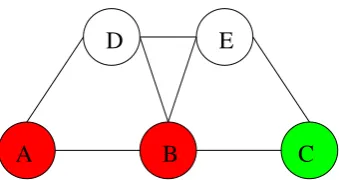
Figure 2.1: Five node network. The red nodesAandB are the source of some network traffic. The green nodeC is the destination of traffic from both source nodes.
lowest-cost path and are thus within the elite selection range. That implies that the number of ants that is generated can be lowered when the number of forward and backward ants is almost equal.
Part II
Chapter 3
Introduction
A big part of the time available for this thesis has been spent on porting the CEAS protocol from ns-2 to ns-3. The following sections provide information about what has been done exactly and the issues encountered along the way. Ns-3 is described in chapter 4, followed by an overview of the design chosen for CEAS in ns-3 in chapter 5. Results obtained from the ns-3 implementation are then validated against the original ns-2 implementation in chapter 6. Finally, chapter 7 discusses the experience of using and extending ns-3.
Chapter 4
About ns-3
This chapter describes the properties of the ns-3 simulator, as presented by the ns-3 developers. In chapter 7, the actual experience with the simulator is discussed.
4.1
Introduction
Ns-3 is a network simulator, developed by mostly the same group of people that work on or have worked on ns-2. It got started because there are problems with the ns-2 design that they felt could not be fixed without breaking compatibility with earlier versions [14].
Specifically, those problems included:
Bi-language system (C++/tcl) Ns-2 uses both C++ and tcl to build sim-ulations. The combination of both languages is difficult to debug and a barrier for new developers.
Scalability problems Tests show that ns-2 does not scale well to large simu-lations, making it unsuitable for some research.
Core packet structure In ns-2, packets are not serialized and deserialized. To be able to run simulations against real-world systems, support for ’real’ packets is needed.
To fix these problems, the ns-3 project was started in 2006. The first stable version was released in June 2008. The current release, as of May 2010, is ns-3.8. New versions are released every three to four months.
4.2
Features
To avoid the problems that developed in ns-2, a number of specific features have been introduced in ns-3. Those are described in the next sections.
Extensible core
Ns-3 is written in C++. It features an optional Python interface. In contrast to ns-2, users don’t necessarily have to know both languages. To make it easy to extend the simulator, its goal is to be documented more consistently than ns-2. Also, the coupling between different models has been minimized by using object aggregation.
Attention to realism
In ns-3, nodes in the simulation resemble real computers more than in ns-2. Every node is constructed out of devices and there is an internet protocol stack that closely resembles the stack on real systems. Applications written in ns-3 can use an implementation of the BSD socket API.
Software integration
Compared to ns-2, it has become easier to interact with other software packages. Network traffic generated by ns-3 can be traced and written to a file in the pcap format, which makes it possible to analyze it with tools like Wireshark.
Support for virtualization and testbeds
Tracing and statistics
In ns-3, a tracing framework makes it possible to decouple tracing as much as possible from the simulation code itself. The code can provide tracing hooks, which can then be connected to tracing sinks by the user. A tracing hook can be the arrival of a packet, the occurence of a certain error state or anything else. Tracing sinks can analyze the incoming data, aggregate it and store it in different formats, depending on the needs of the user.
A statistics module is also included in ns-3, though its current feature set is rather limited. As part of this thesis, the functionality has been extended.
Architecture
Ns-3 consists of a core simulator part and a number of layers that add the networking-specific elements. It provides an internet stack with implementa-tions of protocols like TCP and UDP, as well as lower-level protocols like vari-ous versions of 802.11. Different components and applications can be added to nodes, after which nodes can be connected to each other. To help with build-ing up nodes and creatbuild-ing a network topology, helper scripts are provided. A schematic view of ns-3 is shown in figure 4.1.
Tracing Loging Callbacks Smart pointers
Attributes Random variables Dynamic type system
Events Schedulers Time artithmetic
Mobility models (static, random walk, etc.) Packets
Packet tags Packet headers Pcap/Ascii file writing NetDevice ABC Address types (IPv4, MAC, etc.) Queues
Socket ABC IPv4/IPv6 ABCs Packet sockets Node class High−level wrappers for everything else. Aimed at scripting.
mobility
simulator
core test
helper
internet−stack
routing devices applications
node
[image:28.595.151.497.267.547.2]common
Chapter 5
CEAS in ns-3 - the
architecture
Soon after the thesis project started, it was decided that porting CEAS to ns-3 would be the first step. It was expected that ns-3, being a more modern project and developed by people that knew the advantages and disadvantages of ns-2, would make it easy to extend and improve CEAS. Thus, the time spent on implementing CEAS could be won back by being able to develop improvements in a faster way. In the end, that was not what happened: porting to ns-3 took longer than expected and the extra time could not be compensated by faster development later on.
The CEAS code in ns-3 uses the same algorithms as those used in ns-2. Most of it has, however, been built from scratch in the ns-3 framework. The parts related to the temperature calculations could be taken from ns-2. Some inspira-tion for the design came from the implementainspira-tion of the Optimized Link State Routing (OLSR) protocol, which is the only other decentralized algorithm cur-rently implemented in ns-3. The first part of this chapter describes how the ns-3 version of CEAS is designed. The last section is dedicated to the infrastructure used to perform simulations with ns-3 and is not specific to CEAS.
5.1
Overview
NetDevice (incoming) Network layer
Transport and
CeasRoutingProtocol Ant serialization / deserialization Ns−3 routing table entries NetDevice (outgoing) UdpL4Protocol Ipv4L3Protocol Data packet Routing packet Function call Application CEAS UdpSocket Upper layers Lower layers Ant generator Routing table Routing table entries
RouteInput RouteOutput
Figure 5.1: Design of CEAS within the ns-3 framework.
deserialization of ant packets. Figure 5.1 shows how CEAS has been integrated in the ns-3 framework.
5.2
Temperature table
The temperature table, modelled by a class CeasTemperatureTable, provides methods to add temperature entries to a table and retrieve them. Entries are instances of CeasTemperatureTableEntryand have a key, which is by default a source-destination pair, that identify entries in the table. The original default in ns-2 is to use an identifier that specifies the pheromone type. Other key types can easily be added in both the ns-2 and ns-3 implementation.
TheCeasTemperatureTableEntryitself contains both the normal and the elite
temperatureγof a key and the ‘search focus’ρ. The temperatures, instances of
CeasTemperatures, consist of the actual temperatureγ and the parameters a
andb, which are used to updateγ.
5.3
Pheromone table
Ns-3 provides a classIpv4Route, which models IPv4 routing table entries, and methods to create and update those entries. However, the fields in such an entry are not sufficient for CEAS. For that reason, a new class
CeasRoutingTable-Entry has been added. The class uses ns-3’s IPv4 routing table entries where
possible.
CeasRoutingTable
NextHop
Ipv4Route Ceas−
Routing− Table− Entry
CeasRouting− TableEntry
NextHop
Figure 5.2: Routing table elements of the CEAS implementation.
Every entry has a set of NextHops, which are possible next hops to reach the destination. It is possible to ask for aNextHopinstance in two ways:
• Using stochastic routing with the pheromone values as input, as used by normal forward ants.
• Using a random selection of the next hop, where all hops have equal chances, as used by explorer ants.
NextHopis modelled as a wrapper around ns-3’s routing entries. The wrapped
entries are used to store the IPv4 address of the next hop and the outgoing interface address to reach that address. The values that can not be stored in
the Ipv4Route class provided by ns-3, such as the cost for this link and the
pheromone value associated to it, are stored in theNextHopitself.
5.4
Ant packets
In ns-2, contrary to ns-3, packets are not serialized. For that reason, there was no clear definition of the packet format to use for ants in ns-3. An earlier implementation of CEAS in AntPing [16] used the IPv4 route record mechanism, described in [17] to store route information. Disadvantages of that approach are the limited number of hops that can be stored (no more than nine) and the limited amount of information that can be stored (just the IPv4 address). For the ns-3 implementation, a new packet format has been designed that does not have those limitations.
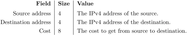
Field Size Value
Source address 4 The IPv4 address of the source. Destination address 4 The IPv4 address of the destination.
[image:32.595.156.483.124.184.2]Cost 8 The cost to get from source to destination.
Table 5.1: Packet structure - hops. Sizes are in bytes.
information that has to be encoded in an ant. This structure has been chosen because it makes it much easier to deserialize ants.
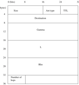
The structure that has been used for normal forward ants is shown in figure 5.3.
Each ’inner’ ant header contains the following fields:
Size (2 bytes) Not used so far.
Ant type (1 byte) Not used so far. This could be used to have different ’types’ of routes between two nodes, for instance one route which has a low latency and another route which is optimized to have a maximal band-width. In that case, the source and destination address are not enough anymore to keep the different ants apart. Note that this field does not specify whether the ant is a forward ant or a backward ant - that is en-coded in the common, ’outer’ header.
TTL (1 byte) The time-to-live (in number of hops) of the packet.
Destination (4 bytes) The IPv4 address of the destination of the packet.
Gamma (8 bytes1) The gamma value of the packet. This is the temperature γ, which is used to update the pheromone values. It is only relevant when the ant is travelling back to its source.
L (8 bytes) The costL of the ant. In the current implementation, it is only relevant when the ant is travelling back to its source. Future extensions could use it to drop a forward ant based on the cost it has accumulated so far.
Rho (8 bytes) The search focusρof the packet. This value is used to update the temperatureγ at the destination.
Number of hops (1 byte) The number of hops the packet has already taken.
Following the ‘number of hops’ field, descriptions of the individual hops are added to the packet. The structure of the description is shown in table 5.1.
Destination
Gamma
L
Rho
Size Ant type TTL
0 (bits)
(bytes)
8 16 24 32
4
8
12
16
20
24
28
32
36
[image:33.595.138.406.265.556.2]Number of hops
The encoding of the different hops the packet has passed deserves some atten-tion. In the current CEAS implementation, both the source and the destination address for each hop are stored in the packet. It is possible to store just the source addresses. However, it is not enough to store just the destination ad-dresses. The reason that the source addresses have to be stored comes from how backward ants find their way. If a forward ant travels from nodeAvia nodeB to node C, a backward ant will be generated at C. This backward ant needs the IP address of the outgoing interface from B to C: that address is used to determine which outgoing interface fromC toB has to be used.
Future extensions to the protocol might need both the source and destination addresses of each hop, for instance when the connections between nodes are not point-to-point links. For that reason and for easier debugging, both the source and destination address have been included in the ants.
For basic CEAS, it is not needed to include the cost of each link: just incre-mentingLat every node on the way would be enough. However, to implement the subpath extension to CEAS, the cost of every hop has to be known. Other extensions might also need the cost of individual hops, so it has been included in the packet structure. However, just like with the other floating point fields, it could be made significantly smaller than it currently is.
Methods have been implemented to change values in a packet, serialize it and deserialize it.
5.4.1
Neighbour discovery packets
In the ns-2 implementation of CEAS, nodes know which neighbours they have. In real networks, that is not necessarily true: neighbours have to be discov-ered somehow. The ns-3 implementation of CEAS contains an extra packet type, called ’hello’ packets, to discover neighbours. Packets are periodically sent through all connected interfaces and when a node receives such a packet, it sends a reply. When a node receives a reply, it adds the sender of the reply packet to the list of known neighbours. If a known neigbour does not reply to a configurable number of discovery packets, it is removed from the list of known neighbours.
A
B
C
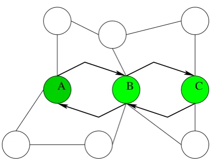
Figure 5.4: Network with nodesA,B andC.
5.5
Routing protocol
Assume a network as shown in figure 5.4. This section describes how the routing protocol is implemented by following a single ant on its way from node A via nodeB to nodeC and back through B toAagain.
5.5.1
Before sending the ants
Before any ants are sent, a basic infrastructure has to be set up. A list of neighbours is needed, as well as a mapping from the IPv4 addresses of the neighbours to the corresponding UDP sockets used to send routing information.
Also, an - initially empty - list of ’needed’ destinations has to be created. This list is used to determine which routes have to be discovered. Using such a list allows for both a reactive and a proactive approach to routing. In the first case, destinations are added when a data packet requests a route to that destination. In the second case, external code can add destinations to the list, which will then automatically be looked for by ants.
5.5.2
Leaving node
A
Ants are generated at regular intervals with a configurable rate. There are separate rates for normal ants and explorer ants. A new ant picks a next hop from the pheromone table. For normal ants, the pheromone values are used to influence the chance of choosing a certain neighbour as the next hop. For explorer ants, every neighbour has an equal chance.
various other fields, such as the time-to-live of the ant, are set to the right values. The packet is then queued for transmission.
When the transmission timer expires, all queued packets are sent. In the current implementation, the transmission timer is set to zero every time a packet is queued. The result is that all packets are sent individually. The timer could be used to send bursts of packets, which might be useful in for instance wireless scenarios.
For every packet that is to be sent, a timestamp is added. This is a tag that is just used for simulation purposes: it is not serialized with the normal packet and thus does not add to the transmission delay. After completing the packet, the socket associated with the link to the next hop is looked up. The packet is then sent through the socket to be processed by the lower layers in the communication stack.
5.5.3
Passing through node
B
When the ant arrives at nodeB, the first part of the header is read. This part contains the identification for the different ant types. Depending on the type of ant, different handling routines are called. In this case, the handler will conclude that the ant has not arrived at its destination yet and that it has to forward it.
Next, some basic checks on the route the ant has taken are performed. The time-to-live should still be above zero and the ant should not have visited the node before. In both cases, the packet is dropped. Then, a next hop for the ant is chosen using the process described before. One difference is that all nodes which have been visited before by the ant are blacklisted: they can not be chosen as a next hop. Note that this does not completely prevent loops: neighbours may have multiple IP addresses, not all of which may be known at B. Thus, the loop check is still needed. Normal forward ant packets are dropped if no valid next hops are found. For explorer ants, that is different: if all neighbours are blacklisted, the blacklist is ignored and the explorer ant is sent to one of the neighbours, where it might find a node which it has not visited yet. The different way to handle explorer ants prevents dropping such ants too often, which would make it difficult to find routes when the discovery process has just started. The ns-2 implementation does not limit this mechanism to explorer ants and handles normal forward ants in the same way.
5.5.4
Arriving at node
C
At C, the packet is analyzed in the same way that happened at B. This time, the system concludes that the ant has arrived at its destination. The temperature valueγis updated for the specific source-destination pair, in this case the route A⇒C. If the route is within certain limits of the best known route, i.e. it is an elite ant (see section 2.2.5), a backward ant is generated.
Backward ants are basically identical to forward ants, except for a field in the header indicating that the ant is on its way back. Thus, the forward ant is simply copied into the new ant and only the first part of the ant is newly generated. The packet is then queued to return toA.
5.5.5
The way back
The ant arrives at node B again, where the pheromone values for all routes to Care updated, based on the values ofγ,L(the cost) andβ. The packet is then forwarded toA, based on the route stored in the ant.
AtA, the same happens, except for the forwarding: it has arrived at its desti-nation and is dropped.
5.6
Infrastructure
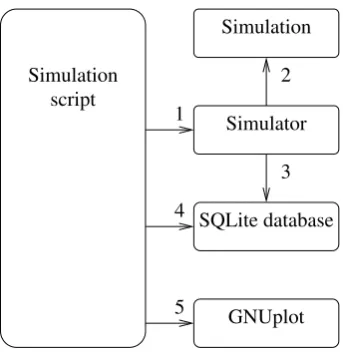
To perform the actual simulation, a number of helper tools have been written. These tools are not specific to CEAS. A simulation run consists of the following steps:
• A simulation script (written in bash/sh) is started.
• The script compiles and runs the simulation scenario file (written in C++) a configurable number of times with the specified options.
• The simulation scenario stores the results in an SQLite database.
• The simulation script runs queries on the SQLite database to get data points.
• The simulation script calls gnuplot to convert the data points to graphs.
Scenario files contain the definition of the network topology and specify any special events, such as link losses, that occur.
Simulation
Simulator Simulation
script
SQLite database
GNUplot 2
3
[image:38.595.237.409.121.299.2]5 4 1
Figure 5.5: Workflow of simulating CEAS with ns-3.
1. The simulation script starts the simulator with specific simulation param-eters.
2. The simulator runs the simulation.
3. The simulator stores the results in a SQLite database after every simula-tion run.
4. The simulation script queries the database to get the results.
5. The results are plotted with GNUplot.
support in the ns-3 interface to SQLite. The problem has been fixed and the resulting patch has been provided to the ns-3 developers2. It is integrated in new ns-3 releases.
To be able to measure the changes in temperature and pheromone values over time, the statistics framework of ns-3 has been extended. Some scripts are used to run a simulation, store the results in a database and extract relevant data from the database to generate graphs. The process is shown in figure 5.5.
2See http://mailman.isi.edu/pipermail/ns-developers/2009-November/006959.html and
Chapter 6
Validation
To assess whether the CEAS port to ns-3 behaves identically to the latest ns-2 version, a number of simulations have been run on both simulators. The results show that the ns-3 code behaves exactly like the original version.
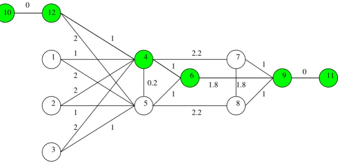
To validate the convergence and temperature calculation, a network consisting of 12 nodes has been chosen. A very similar network has been used in [11] and for the simulation of the subpath extension to CEAS [4]. Because of the experience with the network layout and the available results from ns-2, it was chosen as the network for validating the ns-3 CEAS implementation. In the network, traffic flows from node 10 to node 11. The path with minimal cost is along 10−0−4−6−9−11, which has cost 0.0038s. Figure 6.1 shows the network layout. There is one difference between the network used for ns-3 and the network used before: nodes 10 and 11 have been added. This has been done to have a single interface on both the source and destination node, which makes it easier to run the simulations with the ns-3 implementation. The cost of the links connecting the extra nodes to the original network have been set to zero, so the cost of the path is the same in both networks.
The expected result is that most ants converge to this route. The performance function used in CEAS is h(p, γt) = e−
Lt
γt = ρ (see section 2.2.1). In this
function,Ltthe cost at time t, γt is the temperature at that time andρis the
’search focus’ of the protocol, which is 0.01 in both ns-2 and ns-3. With some rearranging, a theoretical lower bound for the temperature can be found, given values forρand L(dropping the subscript tfor the variables, as this is about the converged state, not an intermediate time):
e−Lγ =ρ
γ=− L
1 2 3 10 12 4 5 6 8 9 11 7 0 1 2 2 1 2 1 2 1 2.2 1 1.8 1.8 1 1 1 0 2.2 0.2
Figure 6.1: The 12-node network used for validation. Costs are delays in mil-liseconds. The shortest path is indicated.
The total temperature γ at node 11 for the source-destination pair (10−11) should gradually converge to − L
ln(ρ). In both simulations, ρ = 0.01 has been used, which gives an expected lower bound for the temperature:
γ=− L
ln(ρ) =− 0.0038
ln(0.01)≈0.000825
Due to explorer ants taking different routes, the temperature of the system will stay slightly higher than 0.000825. The elite temperature, which is only updated by ants with a low enough cost, should always be lower than or equal to the total temperature, but has the same lower bound.
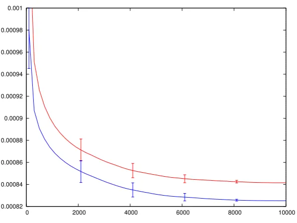
Figures 6.2 and 6.3 show the evolution of temperature over time in ns-2 and ns-3, respectively. The parameters used in the simulation are described in appendix A. The code for updating the temperature has been taken from the ns-2 imple-mentation, so any difference in temperatures between the two implementations comes from other parts of the code.
Figure 6.3 also shows that the elite temperature follows the expected curve: it is always lower than the total temperature, while never getting below the lower bound. The curves from the ns-3 simulation are within the confidence intervals of the curves generated by ns-2.
It was checked manually that the chosen path is indeed 10−0−4−6−9−11: the pheromone values at all intermediate nodes converge to the expected values.
0.00082 0.00084 0.00086 0.00088 0.0009 0.00092 0.00094 0.00096 0.00098 0.001
[image:41.595.137.436.281.505.2]0 2000 4000 6000 8000 10000
Chapter 7
Experience with ns-3
At the beginning of the thesis project, I proposed to use ns-3 instead of ns-2 to run the CEAS simulations. The idea was that it would take more time at first, because of the porting of the protocol to a new simulation, but that it would be possible to make up for that by being able to use a more flexible architecture for all simulations.
In practice, that has not exactly happened. The ns-3 architecture is indeed more flexible and would in theory make it easier to run a large number of different simulations. However, the flexibility is mostly concentrated at the application layer. It is very easy to construct nodes, generate all kinds of network topologies and add applications to nodes. Tracing works well too, though it is slightly less useful because of the lack of a complete statistics module: it is possible to get a lot of information out of the system and it is easy to add hooks to get even more data. However, ns-3 does not offer all the needed components to analyze the data easily. For instance, it is possible to run a simulation with certain input parameters and record the (final) value of whatever is to be measured. However, there is no infrastructure to record how that value changes over time within a simulation.
The most important reason for the delay in porting CEAS to ns-3 is the added realism in the new simulator. In ns-2, nodes can have an ID and packets can simply be sent to a specific node. In ns-3, such a basic operation requires a lot more work:
• The nodes have to run an IP stack, with different IP addresses for every network interface. Thus, there is not a single ’node ID’.
• To send a packet, a TCP or UDP connection has to be established by opening a socket to the destination node. The destination has to have the port open: if not, ICMP error messages will be generated.
pass a structure around in the simulator. Instead, a definition of the packet layout is needed and serialization and deserialization functions have to be written.
The purpose of this research is to improve CEAS, not to get to know the details of the BSD socket API. For that reason, the added realism seems unnecessary - after all, the simulation results show that the ns-2 and ns-3 implementations behave in exactly the same way.
Having said that, there are advantages to the added realism as well. Until now, CEAS did not have a well-defined packet structure. Also, it depended on the existence of a unique identifier for every node, which is not necessarily available in real networks. By forcing realism on the developer, the protocol improves and gets ready for real-world usage. However, for first implementations of a protocol, where the general behaviour is more important than the exact implementation details, ns-3 does not seem the right tool for now.
The experience with implementing a protocol in ns-3 and how it differs from ns-2 has been described in a paper, which is attached to this report as appendix B.
7.1
Comparison with ns-2
7.1.1
Abstraction level
Both ns-2 and ns-3 are packet-based discrete-event simulators, but have different levels of abstraction. Ns-3 mirrors real network components, protocols and APIs more closely. This becomes obvious when implementing CEAS. At the transport and network layers, ns-3 does not abstract any detail. IP and UDP protocols are implemented in detail. A packet is represented as a buffer of bytes and the actual content of a packet needs to be serialized and deserialized. Packets are not simply sent: a socket has to be created and connected and errors have to be handled properly. Trying to connect to a closed port results in an ICMP error message. In ns-2, there is no detailed implementation of either UDP or IP.
As a result, the implementation of the same protocol in ns-2 and ns-3 is signifi-cantly different and porting a protocol from ns-2 to ns-3 is not straightforward.
7.1.2
Usability and adaptability
Elements of usability and adaptability are, among others, how easy it is to learn the tool, to extend existing models and to add new ones. This involves many aspects:
Programming language and debugging
Ns-2 is implemented in C++ and OTcl. Each language taken separately is not difficult to use. The difficulty comes from the combination of the two and the concept of split-object. When developing a new protocol such as CEAS, one has not only to implement objects in both C++ and OTcl, but also the interactions between those objects. This task is made difficult by the lack of documentation and debugging tools for the interface between C++ and OTcl. Ns-3 is written in C++ only and, hence, much easier to debug. It offers Python bindings as well, which are identical to the C++ interface. It is not required to use Python and so far, it looks like most users choose to work with C++.
Building
Unlike ns-2, which uses the traditional GNU build system (autoconf, automake, make), ns-3 uses waf [18]. Waf is a much more recent framework, written in Python, that one needs to learn and adapt to when using ns-3.
Documentation
Existing code
Ns-2 and ns-3 are open-source projects, distributed under the General Pub-lic Licence (GPL). Hence, a way to learn is to read and study existing code. Many models have been contributed to ns-2, but ns-2 code is generally hard to read because: (i) it includes old code for backward compatibility, (ii) many contributions use different coding styles and design approaches and constitute a patchwork of often incompatible models, and (iii) the code is generally poorly commented. In comparison, ns-3 enforces a coding style and a stricter review process before inclusion, which results in more coherent code which is better commented and easier to read. On the other hand, the number of examples is still limited. When the implementation of CEAS in ns-3 was started, the only example of dynamic detailed routing protocol was OLSR.
Modularity
In ns-2, it is not always easy to simply replace a model by another. In the case of routing protocols, models vary depending on the type and numbers of interfaces; see [21]. In ns-3, layers are clearly separated and interfaces well-defined. Replacing objects by similar ones, e.g. a routing protocol, is therefore much easier. On the other hand, the architecture of ns-3 closely maps that of existing systems and implementing untraditional approaches or different levels of abstraction, e.g. abstracting the IP layer, is much more demanding. At the application level, ns-3 is much more flexible than at the transport and network layer.
7.1.3
Built-in components and models
Ns-3’s focus on extensibility makes it easier to add new components and prop-erties to nodes, which can be an advantage. The number of protocols available for ns-3 is still relatively small compared to ns-2. However, new protocols are added regularly, particularly in the field of wireless communications. The in-creased focus on validation makes results obtained with ns-3 potentially more thrustworthy than results from ns-2.
7.1.4
Experiment setup, control and analysis
and distributed execution. For ns-2, several frameworks have been developed and provide some of these features. For ns-3, most of these features are being developed or planned, but not yet integrated.
Furthermore, compared with ns-2, ns-3 provides a powerful framework for trac-ing internal variables, but, for the time betrac-ing, misses generic trace sinks. Other advantages of ns-3 include the use of standard formats, such as pcap for packet tracing, and the integration of interfaces to external software such as SQLite. An effort to improve the data collection framework in ns-3 has been announced in March 2010 [22].
Finally, the support for visualization in ns-2 and ns-3 is limited (Nam and NetAnim, respectively), in particular for wireless networks.
7.1.5
Development status
Ns-2 is funded through the ns-3 project, but the core development team is only working on ns-3. Ns-2 only receives maintenance updates and less and less models are contributed. Ns-3, on the other hand, is under active development. It has been available for developers and early adopters since 2008. Most of the generic building blocks are in place. However, not all the core APIs are completely stable yet, which may keep some developers from moving to ns-3. For example, the routing API has undergone significant changes until version 3.6 (October 2009). One should also expect some rough edges. For instance, during the development of CEAS, it became clear to us that the SQLite output interface was a performance bottleneck and had to be fixed by introducing support for SQL transactions. The resulting patch has since then been integrated.
The original NSF project for ns-3 is ending this year (2010) and a lot has already been achieved. However, referring to the project goals [23], there is still much to do, including porting models from ns-2, providing support for data collection, experiment control and statistic generation, extending the visualization support, and integrating ns-3 with external tools such as Click. Recently, a new NSF grant has been announced for the development of “frameworks for ns-3” [22]. The framework will focus on better support for controlling the execution of simulations and analyzing the results. Finally, part of the development of ns-3 is also founded through the Google Summer of Code (GSoC) [24] program.
7.1.6
Efficiency
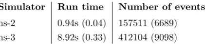
Simulator Run time Number of events
ns-2 0.94s (0.04) 157511 (6689)
[image:48.595.218.429.123.169.2]ns-3 8.92s (0.33) 412104 (9098)
Table 7.1: Performance comparison
spent in the ’added’ layers: those parts that are not included in ns-2, like socket handling and serialization. The detailed implementation of the transport and network layer require processing time, which is not used in ns-2. To compare memory usage, we created 10.000 nodes with an IP stack and the CEAS imple-mentation. Ns-3 used about half as much memory as ns-2. The difference comes from the fact that the ns-3 node is simply a container and only the required components are instantiated while the ns-2 node is a much more static construct including components that may not be used.
Part III
Chapter 8
Simulation
8.1
Introduction
After the implementation and validation of the routing protocol, a scenario has been defined. Based on the scenario, a number of simulations have been run, using different configurations of the protocol.
8.2
The scenario
To have meaningful simulations, a scenario has been defined. Simulations could then be run with the scenario as a basis and any changes could be compared to the basic protocol more easily.
The defined scenario is a city that provides wireless access to its inhabitants. One example of such a city is Trondheim, where wireless access is provided by Tr˚adløse Trondheim [25].
The city has an infrastructure with different base stations and a (potentially large) group of mobile users. The base stations are connected to each other and route the traffic to ’the internet’. Depending on how the users move, the traffic pattern within the network of base stations changes, which might cause congestion in part of the network.
8.2.1
The layout
would fit many other city centers as well. Base stations are placed at regular intervals at some of the bigger streets. The chosen layout affects the simulation results. One characteristic of a grid layout with equal costs for each link is that there are often many paths to a destination with the same cost.
The layout models the location of base stations, not the location of end users. It is assumed that the end user equipment will select the base station it connects to automatically. As the user moves around, his or her equipment will switch base stations as necessary. Thus, base stations will transfer fluctuating amounts of data, depending on what traffic users generate and how they move around. The generated traffic depends on the services that users use and how those services are used. Base stations are connected by point-to-point links with a delay of 500ns between base stations. This value has been chosen because standard Cat5 ethernet cables have a delay of about 5ns/m, resulting in a simulated distance between base stations of about 100 meter. How users are connected to the base station does not infuence the results and has not been specified in the simulations. Given the scenario, a wireless connection should be expected. It is assumed that users are connected to at most one base station at a time, which is true for standard WiFi connections.
All links between base stations are simulated at a bandwidth of 1M bps. That is a lower bandwidth than can be expected in reality. The low bandwidth is used to limit the number of packets that has to be simulated to congest a link. With higher bandwidths, the number of packets that has to be simulated grows, and so does the simulation time in ns-3. The effect can be limited by using bigger packets, but that has limitations as well: UDP packets have a size limit, which means that packets have to be split and the total number of packets grows again. It has been tested that a link of 1M bpsprovides more than enough bandwidth to make the effect of CEAS packets on available bandwidth disappear completely: routing traffic uses a few kilobits per second at the very most, or less than one percent of available bandwidth.
Instead of simulating every end user, simulations are limited to simulating the network of base stations. The movement of users is simulated by changing the amount of traffic each base station generates. That way, the processing power needed for the simulation can be limited. Because end users are assumed to send all data to the base stations (i.e. no other networks are involved), the simulation should give the same results as a simulation including all the end users would.
5
9
13 1
8
12
16 4
7
11
15 3
6
10
[image:53.595.100.445.126.376.2]14 2
Figure 8.1: Trail through 16-node grid network. The red node is the start position of the traffic source. The source then follows the arrows to different nodes, moving every 1000s. The green node is the destination of all generated traffic.
8.3
Basic results
The first simulations test how the system behaves when a user moves through the system.
In this simulation, no background traffic is generated at all and every base station has to start looking for a route to the destination when the user starts to use that base station. Once a destination has been requested, the base station will maintain the route - even if it is not requested again. As such, it is not completely realistic yet, but it provides a good way to see whether the scenario shows the expected behaviour. In this case, the expected behaviour is that the delay to the destination is directly proportional to the distance in number of hops to that destination. Also, the delay is expected to show a spike when the user arrives at a new base station. That spike comes from the time it takes to converge to the shortest route.
0 5000 10000 15000 20000 25000 30000 35000 40000
0 1000 2000 3000 4000 5000 6000 7000 8000 9000
Average delay (microseconds) --- average of 30 trials
Time (s)
Delay over time in 16-node network
[image:54.595.159.491.131.366.2]CEAS Default, beta = 0.95, no background traffic
Figure 8.2: Delay over time - basic scenario.
and does not include routing packets. The parameters for the simulation are described in appendix A.
The next step is to include background traffic. The background traffic is a traffic flow which uses a significant part of the bandwidth along the dashed line in figure 8.3. The background traffic is enabled at t = 3000s. From then on, some paths to the destination are loaded and have a higher queueing delay. At all times, there is a route which is fast (in number of hops) and not loaded -except for 6000s≤t <7000s, when the single shortest route is loaded.
5
9
13 1
8
12
16 4
7
11
15 3
6
10
[image:55.595.185.359.121.300.2]14 2
Figure 8.3: Trail through 16-node grid network with background traffic along the dashed line. Again, the red node is the start position of the traffic source and the green node is the destination of all generated traffic.
the link is again overloaded and the average delay will return to its old value and grow again.
8.4
Load-sensitive cost functions
To improve the situation with loaded links, a cost function which is load-sensitive has been added to the protocol. To be able to do that, the load of a link is estimated. The estimation formula used is:
newTrafficRate = smooth×oldTrafficRate +
(1.0−smooth)×currentTrafficRate
The current traffic rate is estimated by receivedBits
10000 100000 1e+06 1e+07 1e+08
0 1000 2000 3000 4000 5000 6000 7000 8000 9000
Average delay (microseconds) --- average of 30 trials
Time (s)
Delay over time in 16-node network
[image:56.595.160.490.131.366.2]CEAS Default, beta = 0.95, with background traffic
Figure 8.4: Delay over time - with background traffic from t = 3000s. The delay of the background traffic itself is not included in the calculation. Note the logarithmic scale of the y-axis: the delay does in fact grow linearly.
Without the smoothing mechanism, traffic rates could easily seem to be higher than the link capacity, simply because a few big packets were added to the queue in a short period. An extreme example would be a 50kbit packet, which is queued every 10 seconds on a 10kbps link. Clearly, the link is just used at half of its capacity - but without the smoothing parameter, the link would seem overloaded once every ten seconds and completely idle for the other nine sec-onds. Though seemingly unrealistic, similar situations actually occured during simulations with CEAS.
Implementing this estimation uncovered bugs in ns-3: the functions that were supposed to return the number of queued bytes and packets did not work prop-erly. The problem has been solved; patches have been sent to the developers and have been added to the newest release of ns-31.
Given the estimation of the traffic rate, the loadρis defined aslink capacity (bits/s)traffic rate (bits/s) , or λ
µ in variables from queueing theory. Note that this is a differentρthan the
parameter used in CEAS.
The first load-sensitive cost function is 1−1ρ, which has the properties that are desired in such a function: it returns a low cost when the load is low and it grows as the load gets higher. In this case, the cost goes to infinity as the load reaches the link capacity.
1See http://mailman.isi.edu/pipermail/ns-developers/2009-December/007144.html and
5000 10000 15000 20000 25000 30000 35000 40000 45000
0 1000 2000 3000 4000 5000 6000 7000 8000 9000
Average delay (microseconds) --- average of 30 trials
Time (s)
Delay over time in 16-node network
[image:57.595.111.440.131.365.2]CEAS Default, beta = 0.95, no background traffic CEAS Cost 1, beta = 0.95, background traffic
Figure 8.5: Delay over time with load-sensitive cost function. For comparison, the normal CEAS without background traffic has been included as well.
The resulting plot of using such a cost function can be seen in figure 8.5. When there are no congested links, the delay converges to the lowest possible delay. From t = 3000s, when some of the links are congested, part of the traffic is sent along a different path, resulting in a slightly higher end-to-end delay - but nothing like the delays seen with hop count as the cost metric.
Based on this result, simulations have been run with similar functions, but with a steeper curve - like 1
(1−ρ)2. The goal was to have a function which would react even faster on overloaded links by having a bigger difference in cost between loaded and unloaded links. However, those functions did not perform better than the cost function used in figure 8.5.
A different way of assigning a cost to a certain load is the following:
cost = ρ
totalBandwidth−usedBandwidth
Withρ= usedBandwidth totalBandwidth =
λ
µ. A plot of both functions is shown in figure 8.6.
0 2 4 6 8 10
0 0.2 0.4 0.6 0.8 1
Cost
Load (%) Cost functions
[image:58.595.157.487.129.364.2]First cost function Second cost function
Figure 8.6: Cost as a function of link load for the first two cost functions.
Thus, the system would converge to the loaded link. In practice, that might not be bad, because the loaded link (given the low cost of 2) would still have a lot of capacity left - but for complete avoidance of loaded links, the second cost function would seem like a good candidate.
The resulting plot, shown in figure 8.7 shows that the second load-sensitive cost function does work, but in an unintended way. The relative cost difference be-tween two paths at a low load is already high, which causes the system to keep switching to the lowest loaded path it can find, without taking the length into account. Thus, the system does not converge to the shortest path. The advan-tage is that an overloaded link will not change the end-to-end delay significantly: because the traffic is always balanced over different paths, only part of the traffic will be affected and the average delay will not change much. Of course, that’s not very useful if that average delay is higher than the maximum delay that other cost functions return. The second cost function is not an improvement over the first function.
A third cost function usesλandµto estimate the mean waiting time and uses that as a cost value:
cost = 1
totalBandwidth−availableBandwidth = 1 µ−λ
0 10000 20000 30000 40000 50000 60000 70000 80000
0 1000 2000 3000 4000 5000 6000 7000 8000 9000
Average delay (microseconds) --- average of 30 trials
Time (s)
Delay over time in 16-node network
[image:59.595.107.441.133.366.2]CEAS Default, beta = 0.95, no background traffic CEAS Cost 2, beta = 0.95, background traffic
Figure 8.7: Delay over time with second load-sensitive cost function. For com-parison, the normal CEAS without background traffic has been included as well.
should be a reasonable estimate of the expected waiting time in the real world.
As shown in figure 8.8, the third cost function performs very similar to the first cost function. In fact, it is not just ’very similar’: the results of the two cost functions are identical. It is not difficult to see why that happens. The first cost function is:
1 1−ρ
That cost function can be shown to be equal to the third cost function, except for a constant factor:
1 1−ρ =
5000 10000 15000 20000 25000 30000 35000 40000 45000
0 1000 2000 3000 4000 5000 6000 7000 8000 9000
Average delay (microseconds) --- average of 30 trials
Time (s)
Delay over time in 16-node network
[image:60.595.159.491.130.364.2]CEAS Default, beta = 0.95, no background traffic CEAS Cost 3, beta = 0.95, background traffic
Figure 8.8: Delay over time with third load-sensitive cost function. For compar-ison, the normal CEAS without background traffic has been included as well.
1
1−ρ =
1 1−λ
µ
= µ
µ∗ 1 1−λ
µ
= µ∗ 1
1−(λµ)∗µ
= µ∗ µ1 −λ
8.5
Preplanning
In the simulations so far, the routing protocol has been purely reactive: a node only starts to look for a route when there is a direct demand for it from a traffic source on that node. From then on, it will keep the route updated indefinitely.
Another approach is to use some type of proactive approach: routes are already discovered before they are requested. The advantage is that, when a request comes up, it should take less time - or even no time at all - to converge to the shortest route. The clear disadvantage is the extra overhead: ants will be sent to discover routes that will never be used. Whether the faster convergence is desirable enough to outweigh the overhead depends on the situation. In relatively static networks with many traffic sources, it makes sense to discover routes proactively: they would have to be discovered at a later time anyway, so it makes sense to do it in time and prevent unnecessary delays. In more dynamic networks with less traffic sources, it is probably not a good idea, because the chance that a route will actually be needed is smaller. On top of that, there is a bigger chance that a route which has been discovered before is not available anymore due to changes in the network topology: in that case, the ’investment’ of finding a route early is lost and there will be a delay to find a new, working route anyway.
The CEAS implementation in ns-3 makes it possible to use preplanning. One approach is to discover routes to those hosts that any ’passing’ data traffic has as its destination. The idea is that those destinations are relatively likely to be requested later on anyway, so it might pay off to look for routes to them. The results for preplanning those routes is shown in figure 8.9. As can be seen, the peaks that were visible when a user moved to a new base station have disappeared. That is the expected effect: routes have already been discovered when the user arrives, so no time is needed to converge to the shortest route.
8.6
Packet format improvements
The CEAS packet format as described in section 5.4, especially figure 5.3 and table 5.1, makes it easy to add new features to the protocol and test extensions such as subpaths (see subsection 2.2.5). However, it is not optimized for effi-ciency. A simple potential improvement to the protocol would be to use a more compact packet format. A suggestion for such a format is shown in table 8.1. Note that, contrary to the improvements mentioned in the last two sections, no simulations have been run with the compact format.
The encoding for each hop can be done as described in table 8.2.
0 5000 10000 15000 20000 25000 30000 35000 40000
0 1000 2000 3000 4000 5000 6000 7000 8000 9000
Average delay (microseconds) --- average of 30 trials
Time (s)
Delay over time in 16-node network
[image:62.595.157.491.143.373.2]CEAS Default, beta = 0.95, pre-planned
Figure 8.9: Delay over time with preplanning. The peaks when moving to a dif-ferent base station, seen in simulations without preplanning, have disappeared.
Field Normal size (bytes) Compacted size (bytes)
Size 2 0
Ant type 1 0
TTL 1 1 (or a few bits)
Destination 4 4
Gamma 8 1
L 8 1
Rho 8 1
Number of hops 1 1
[image:62.595.152.471.426.578.2]Total size 33 9
Table 8.1: Compact packet structure - changed fields in italic.
Field Normal size (bytes) Compacted size (bytes)
Source address 4 4
Destination address 4 0
Cost 8 0
Total size 16 4
[image:62.595.152.491.618.695.2]structure. In that case, a value likeγwould not have to be stored in a forward ant, resulting in an even smaller forward ant packet.
In the scenarios simulated in this report, the smaller packets will not make a significant difference: the link capacity and speed of any modern link will not show any measurable difference between packets of 31 or 123 bytes. Only in very specific situations, the difference might become significant. Such situations would include networks with narrow or very unstable links: in that case, smaller packets might have a higher chance of being transmitted successfully and a lower chance of causing congestion. In most cases, limiting the amount of ants will be much more effective than
Chapter 9
Conclusion
9.1
The original plan
The goal of this thesis project, as stated at the start of it, was to extend CEAS for use in dynamic networks, in which the network topology or other circum-stances change regularly. Would it be possible to adapt CEAS for such envi-ronments? And if so, what would have to be changed? Those changes would then be simulated to verify that the system would indeed work in dynamic environments.
Already at the beginning of the project, it was decided to implement CEAS in ns-3, instead of using the existing ns-2 implementation. The idea was that ns-3 would be easier to learn and to extend - resulting in faster improvements to CEAS once the implementation would be complete. Thus, the plan became to:
• Implement CEAS in ns-3
• Verify the implementation against the existing ns-2 implementation
• Come up with improvements to CEAS for use in environments with a relatively high rate of changes in the network topology
• Simulate the improvements to verify them
9.2
What actually happened
faster later on, became a more important part of it. The first two items of the list above have been realized: CEAS has been implemented in ns-3 and the implementation has been verified.
The other two items, related to the improvement of CEAS, have been done to a smaller extend. Improvements have been proposed for one specific aspect of dynamicity in networks: congestion. The protocol has been adapted to behave in a better way in congested networks, while still showing good behaviour in networks where congestion is no issue.
Though the last items on the list have not been investigated as deeply as planned, some extra work has been done instead. Having CEAS implemented in both ns-2 and ns-3 allowed for a comparison between the two simulators. As it looks likely that both ns-2 and ns-3 will be used for some time to come, the comparison is interesting for anyone having to decide which simulator to use for his or her research. Together with Laurent Paquereau and Poul Heegaard, a paper has been written that describes the experience with both simulators. Our findings have been presented at a PhD course at NTNU and will be presented at SIMUL 2010.
Experience with ns-3
From the experience gained by implementing CEAS, ns-3 is a promising tool. It relies on good programming practices and provides carefully designed generic building blocks which make it easily extensible. Although some APIs are not fully stable yet, ns-3 is in many respects ready for active use and is to replace ns-2 as more and more models are added to it. The development of a framework for data collection and experiment control for ns-3 will also be a strong argument for moving to ns-3. One challenge remains maintaining the documentation and improving its coverage.
Whether to already take ns-3 in use depends on several criteria, including earlier e
![Figure 4.1: Schematic view of ns-3 architecture, based on figure from [15].](https://thumb-us.123doks.com/thumbv2/123dok_us/1204475.643952/28.595.151.497.267.547/figure-schematic-view-ns-architecture-based-gure.webp)