Bootstrap Domain-Specific Sentiment Classifiers from Unlabeled Corpora
Andrius Mudinas, Dell Zhang, and Mark Levene Department of Computer Science and Information Systems
Birkbeck, University of London London WC1E 7HX, UK
[email protected],[email protected],[email protected]
Abstract
Thereisoftentheneed toperformsentiment classificationinaparticulardomainwhereno labeleddocument isavailable. Although we couldmakeuseof ageneral-purpose off-the-shelfsentimentclassifierorapre-builtonefor adifferentdomain,theeffectivenesswouldbe inferior.Inthispaper,weexplorethe possibil-ityofbuildingdomain-specificsentiment clas-sifiersw ithu nlabeledd ocumentso nly.Our investigation indicates that in the word em-beddings learned from the unlabeled corpus ofagivendomain, thedistributedword rep-resentations(vectors)foroppositesentiments form distinct clusters, though those clusters are not transferable across domains. Ex-ploiting such a clustering structure, we are able to utilize machine learning algorithms to induce a quality domain-specific senti-ment lexicon from just a few typical senti-mentwords(“seeds”). An importantfinding isthat simplelinear model based supervised learning algorithms (such as linear SVM) can actually work better than more sophis-ticated semi-supervised/transductivelearning algorithms which represent the state-of-the-arttechniqueforsentimentlexiconinduction. Theinducedlexiconcouldbeapplieddirectly inalexicon-basedmethodforsentiment clas-sification,butahigherperformancecouldbe achieved througha two-phase bootstrapping methodwhichusestheinducedlexiconto as-signpositive/negativesentimentscoresto un-labeled documentsfirst,a ndt henu sesthose documentsfoundtohaveclearsentiment sig-nals as pseudo-labeled examples to train a documentsentiment classifierv iasupervised learningalgorithms(suchasLSTM).On
sev-eral benchmark datasets for document senti-ment classification, our end-to-end pipelined approach which is overall unsupervised (ex-cept for a tiny set of seed words) outper-forms existing unsupervised approaches and achieves an accuracy comparable to that of fully supervised approaches.
1 Introduction
Sentiment analysis (Liu, 2015) is a popular research topic which has a wide range of applications, such as summarizing customer reviews, monitoring social media, and predicting stock market trends (Bollen et al., 2011). A basic task in sentiment analysis is to classify the sentiment polarity of a given piece of text (document), i.e., whether the opinion expressed in the text is positive or negative (Pang et al., 2002), which is the focus of this paper.
There are many different approaches to senti-ment classification in the Natural Language Process-ing (NLP) literature — from simple lexicon-based methods (Ding et al., 2008; Thelwall et al., 2010; Thelwall et al., 2012) to learning-based approaches (Pang and Lee, 2004; Turney, 2002; Jo and Oh, 2011; Argamon et al., 2007; Lin and He, 2009), and also hybrid methods in between (Mudinas et al., 2012; Zhang et al., 2011). No matter which ap-proach is taken, a sentiment classifier built for its target domain would work well only within that spe-cific domain, but suffer a serious performance loss once the domain boundary is crossed. The same word could drastically change its sentiment polarity (and/or strength) if it is used in a different domain. For example, being “small” is likely to be negative
269
for a hotel room but positive for a digital camcorder, being “unexpected” may be a good thing for the end-ing of a movie but not for the engine of a car, and we will probably enjoy “interesting” books but not nec-essarily “interesting” food. Here, the domain could be defined not by the topic of the documents but by the style of writing. For example, the meanings of words like “gay” and “terrific” would depend on whether the text was written in a historical era or modern times.
When we need to perform sentiment classifica-tion in a new domain unseen before, there are usu-ally neither labeled dictionary available to employ lexicon-based sentiment classifiers nor labeled cor-pus available to train learning-based sentiment clas-sifiers. It is, of course, possible to resort to a general-purpose off-the-shelf sentiment classifier, or a pre-built one for a different domain. However, the ef-fectiveness would often be unsatisfactory because of the reasons mentioned above. There have been some studies on domain adaptation or transfer learn-ing for sentiment classification (Blitzer et al., 2007; Tan et al., 2009; Pan et al., 2010; Glorot et al., 2011; Yoshida et al., 2011; Bollegala et al., 2013; Xia et al., 2013; Yang and Eisenstein, 2015), but they still require a large amount of labeled training data from a fairly similar source domain, which is not always feasible. Those algorithms also tend to be computational-expensive and time-consuming (Mo-hammad and Turney, 2010; Fast et al., 2016).
In this paper, we propose an end-to-end pipelined
nearly-unsupervised approach to domain-specific
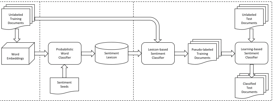
sentiment classification of documents for a new domain based on distributed word representations (vectors). As shown in Fig. 1, the proposed approach consists of three main stages (components):
(1) domain-specific sentiment word embedding, (2) domain-specific sentiment lexicon induction, (3) domain-specific sentiment classification of
doc-uments.
Briefly speaking, given a large unlabeled corpus for a new domain, we would first set up the vector space for that domain via word embedding, then induce a sentiment lexicon in the discovered vec-tor space from a very small set of seed words as well as a general-purpose lexicon, and finally exploit the induced lexicon in a lexicon-based document sentiment classifier to bootstrap a more effective
learning-based document sentiment classifier for that domain. The second stage of our approach out-performs the state-of-the-art unsupervised method for sentiment lexicon induction (Hamilton et al., 2016), which is the most closely related work (see Section 2). The key to the superior performance of our method compared with theirs is the insight gained from our first stage that positive and neg-ative sentiment words are largely clustered in the domain-specific vector space but these two clus-ters have a non-negligible overlap, therefore semi-supervised/transductive learning algorithms could be easily misled by the examples in the overlap and would actually not work as well as simple super-vised classification algorithms. Overall, the docu-ment sentidocu-ment classifier resulting from our nearly-unsupervised approach does not require any labeled document to be trained, and it can outperform the state-of-the-art unsupervised method for document sentiment classification (Eisenstein, 2017). The source code for our implemented system and the datasets for our experiments are open to the research community1.
The rest of this paper is organized as follows. In Section 2, we review previous studies on this topic. In Sections 3 to 5, we describe the three main stages of our approach respectively. In Section 6, we draw conclusions and discuss future work.
2 Related Work
Most of the early sentiment analysis systems took lexicon-based approaches to document sentiment classification which rely on pre-compiled sentiment lexicons (Owsley et al., 2006). Various methods have been proposed to automatically produce such sentiment lexicons (Hu and Liu, 2004; Ding et al., 2008). Later, the focus of research shifted to learning-based approaches (Pang et al., 2002; Pang and Lee, 2004), as supervised learning algorithms usually deliver a much higher accuracy in senti-ment classification than pure lexicon-based meth-ods. However, lexicons have not completely lost their attractiveness: they are usually easier to un-derstand and to maintain by non-experts, and they can also be integrated into learning-based sentiment classifiers (Mudinas et al., 2012; Eisenstein, 2017).
Unlabeled Training Documents
Word Embeddings
Sentiment Lexicon
Pseudo-labeled Training Documents Probabilistic
Word Classifier
Sentiment Seeds
Lexicon-based Sentiment
Classifier
Learning-based Sentiment
Classifier Unlabeled
Test Documents
[image:3.612.77.543.53.226.2]Classified Test Documents
Figure 1: Ournearly-unsupervisedapproach todomain-specificsentiment classification.
The lexicon-based sentiment classifier used in our experiments is a publicly-available system called pSenti2 (Mudinas et al., 2012). In addition to a customizable sentiment lexicon, it also uses shallow NLP techniques like part-of-speech (POS) tagging and the detection of sentiment inverters and other modifiers (intensifying and diminishing adverbs).
The introduction of modern word embedding techniques like word2vec (Mikolov et al., 2013) and GloVe (Pennington et al., 2014) have opened the possibility of new sentiment analysis methods. Given a large unlabeled corpus, such techniques can learn from word co-occurrence information and pro-duce a vector space of hundreds of dimensions, with each word being assigned a corresponding vector. The resulting vector space helps in understanding the semantic relationships between words and al-lows grouping of words based on their linguistic similarities. Recently Rothe et al. (2016) proposed the DENSIFIER method that can reduce the dimen-sionality of word embeddings without losing seman-tic information and explored its application in vari-ous domains. For the SemEval-2015 task (Rosenthal et al., 2015), DENSIFIER performed slightly worse compared to word2vec, though its training time was shorter by a factor of 21. In fact, previous studies such as (Rothe et al., 2016; Cliche, 2017) suggest that word2vec usually provides the best word em-beddings for sentiment analysis tasks.
In their recent work, Hamilton et al. (2016)
2https://goo.gl/pj4XAQ
demonstrated that by starting from a small set of seed words and conducting label propagation over the lexical graph derived from the pairwise prox-imities of word embeddings, they could induce a domain-specific sentiment lexicon comparable to a hand-curated one. Intuitively, the success of their method named SentProp requires a relatively clear separation between sentiment words of opposite po-larity in the vector space which, as we will show later, is not very realistic. Moreover, they have fo-cused on the induction of sentiment lexicons alone, while we are trying to design an end-to-end pipeline that can turn unlabeled documents in a new do-main directly to their sentiment classifications, with domain-specific sentiment lexicon induction as a key component.
4096 units, despite the fact that the LSTM was only trained for a completely different purpose — to pdict the next character in the text of Amazon re-views. Our results are in line with those findings and confirmed the superiority of LSTM in building document-level sentiment classifiers.
Zhang et al. (2011) tried to address the low re-call problem of lexicon-based methods for Twitter sentiment classification via training a learning-based sentiment classifier using the noisy labels generated by a lexicon-based sentiment classifier (Ding et al., 2008). Although the basic idea of their work is similar to what we do in the third stage of our ap-proach (see Section 5), there exist several notable differences. First, they adopted a single general-purpose sentiment lexicon provided by Ding et al. (2008) and used it for all domains, while we would induce a different lexicon for each different domain. Consequently, their method could have a relatively large variance in the document sentiment classifica-tion performance because of the domain mismatch (e.g., F1 = 0.874 for the “Tangled” tweets and
F1 = 0.647for the “Obama” tweets), whereas our
approach would perform quite consistently over dif-ferent domains. Second, they would need to strip out all the previously-known opinion words in their single general-purpose sentiment lexicon from the training documents in order to prevent the training bias and force their document sentiment classifier to exploit domain-specific features, but doing this would obviously lose the very valuable sentiment signals carried by those opinion words. In contrast, we would be able to utilize all terms in the training documents, including those opinion words that ap-peared in our automatically induced domain-specific lexicons, as features, when building our document sentiment classifiers. Third, they designed their method specifically for Twitter sentiment classifica-tion, while our approach would work for not only short texts such as tweets (see Section 5.2) but also long texts such as customer reviews (see Sec-tion 5.1). Fourth, they had to use an intermediate step to identify additional opinionated tweets (ac-cording to the opinion indicators extracted through theχ2 test on the results of their lexicon-based
sen-timent classifier) in order to handle the neutral class, but we would not require that time-consuming step as we would use the calibrated probabilistic outputs
of our document sentiment classifier to detect the neutral class (see Section 5.3).
3 Domain-Specific Sentiment Word Embedding
Our approach to domain-specific document-level sentiment classification is built on top of word em-beddings — distributed word representations (vec-tors) that could be learned from an unlabeled corpus to encode the semantic similarities between words (Goldberg, 2017).
In this section, we investigate how the embed-dings of sentiment words for a particular domain would look like in the domain-specific vector space. To ensure a fair comparison with the state-of-the-art sentiment lexicon induction technique SentProp3 (Hamilton et al., 2016) later in Section 4, we adopt the same publicly-available pre-trained word em-beddings for the following three domains together with the corresponding sets of sentiment words (i.e., sentiment lexicons).
• Standard-English. We use the the Google News word embeddings4and the ‘General Inquirer’ lex-icon (Stone et al., 1966) with the sentiment polar-ity scores collected by Warriner et al. (2013).
• Twitter. We use the word embeddings constructed
by Rothe et al. (2016) and the sentiment lexicon from the SemEval-2015 Task 10E (Rosenthal et al., 2015).
• Finance. We use the word embeddings learned
us-ing an SVD-based method (Mannus-ing et al., 2008) from a collection of “8-K” financial reports5(Lee et al., 2014) and the finance sentiment lexicon hand-crafted by Hamilton et al. (2016).
Note that the above three sentiment lexicons would be used for both the inspection of sentiment word distributions in this section and the evaluation of sentiment lexicon induction later in the next sec-tion. Furthermore, to facilitate a fair compari-son with the state-of-the-art unsupervised document sentiment classification technique ProbLex-DCM6 (Eisenstein, 2017) later in Section 5, we also adopt the following two document collections which they have used.
• IMDB. We use 50k movie reviews in English from IMDB (Maas et al., 2011) with 25k labeled training documents.
• Amazon. We use about 28k product reviews in English across four product categories from Ama-zon (Blitzer et al., 2007; McAuley and Leskovec, 2013) with 8k labeled training documents. The word embeddings for the above two domains
were trained by us on the respective corpora
us-ing word2vec (Mikolov et al., 2013) which employs a two-layer neural network and is by far the most widely used word embedding technique. Specifi-cally, we ran word2vec with skip-gram of a five-word window to construct five-word vectors of 500 di-mensions, as recommended by previous studies7. The sentiment lexicon made by Liu (2015) is consis-tently one of the best for analyzing reviews (Ribeiro et al., 2016), so it is used for both of those domains. Drawing an analogy to the well-knowncluster
hy-pothesisin Information Retrieval (IR) (Manning et
al., 2008), here we put forward the cluster hypothe-sis for sentiment analyhypothe-sis: words in the same cluster behave similarly with respect to sentiment polarity in a specific domain. That is to say, we expect pos-itive and negative sentiment words to form distinct clusters, given that they have been represented in an appropriate vector space. To verify this hypothesis, it would be useful to visualize the high-dimensional sentiment word vectors in a 2D plane. We have tried a number of dimensionality reduction tech-niques including thet-distributed Stochastic Neigh-bor Embedding (t-SNE) (van der Maaten and Hin-ton, 2008), but found that simply using the clas-sic Principle Component Analysis (PCA) (Bishop, 2006) works very well for this purpose.
We have found that in general, the above cluster hypothesis holds for word embeddings within a spe-cific domain. Fig. 2a shows that in the Standard-English domain, the sentiment words with opposite polarities would form two distinct clusters. How-ever, it can also be seen that those two clusters would overlap with each other. That is because each word carries not only a sentiment value but also its linguis-tic and semanlinguis-tic information. Zooming into one of the word vector space regions (Fig. 2b) can help us understand why sentiment words with different
po-7https://goo.gl/SyAdej − − + + − − − − + + + + − − − − − + − − + − − − + − + − + − − − + + + + − + − − − + + + + − + + − + + − + − − + − − − + − − − + + − − + + − + − + − + − + − + + + − + + − + − + − − + − − − + + − − − − − + − − − − − + − − − + − + + − + + + + − + + − + − − − − − + + + + + + − − − − + − − − + − − − − + − + − − − − + + − + + + − + − + − − − − + − − + + + + − − + − + − − − + + + + − − − − − + − + + + − − + − − − − − − + + − − + − − + + − − − + + − − − + − − + − − + − − + − − + + + + − − − − − − − + − − + − − − − − + − − − + − + − + + + + + + − − − − − + − − − − + ++ − − + − + + − − − + + + − − + + + − − − − − + + + + + − + + − − − + + − − + − − − − + − − + − + − − + − + − − + − − − − − − + − − − − − + − − − − − − − − − + − + +− + − − − − + − − + + + − − + − − + + + − − − + − − + − + + + + − + + + + + − − − − + − + + + − − + + − − − + − + − − − + + − + − + + + − − − − − − + − + − − − − − + − − − − − − − + − + − + + − − − − − − − − − + − + − + − − + + − − − − − + − − + + + − + + − − − + + − + − − − − − − − − − − − − − − − + − − + − + − + − + + + − − − − − − + − − − − − − − − − − − + − − − + + − − − + − − − − + − + + + − − − + − + − − − + − + − − + − + − − − − − + + − + + − + − − − + − − + + − + + − − − − − − + − − − − + + − + + + − − + + + + − + + − − + + − + + − − − + + − + − − − + + − − − − + − + − − − + − + − + − − − + + − − + − + + − + + − − + + + + − + − + − − − + − + − + − − − − − + + + + − + − + − + + − − + + − + + − − + − − + − − − − + + − − + − − − − + − + + + − + + − + − + + + − − − − − − + − − − − − − − − − − + − + − + − − + − − + − − + + − + − + − − + − − − − + − + − − + − + − − + − + − − − + − − + − − − − − + + + + − + − − − + − − + − − + − − − − − − − − − + − + − − − − − − − − + − + − + + + − + − − − + + − − − − − + − + − + + − − − − − − − − + + − − − + − − − + − − − + − + − + − − − − − − + + + − + − − + − + + + − + − − − + + + − + − − + − − − − + + − − + − − − − − − − + − + − − − + − + + − + − − − − + − − − − + − + + − + + + − + − − − − − − − + − + + + − + + + − − + − − − − + − − − − + − + − − − + − + − + + − + + − + − − − − + + − − − − + − + − − − + + + − − − + + − − + − − − − − + − + + − − + − − − − − − − − − − + − − − + − − + − + − − + − + − − − − − − − + + + + + + + − + − − − − − + − − + − + − − − + − − + + + − − + − + + − − − − − − − − + − + − − − − − − − + − − + − + + − − + + − − + − − − − − − − − − − + − + − + − + − − + − − − − − − − + − + + − + − − + + − − − − − − − − + − + − − + − − − − − + + − − + + + − − − + − − + − − + + − + + − − + − + + + + − + − − − − + + − + − − + − + + − − + + − + − − − − + − − + + − − + − − − − + − − − + − + − − + − − − + + − + − − − + − + − + − − + − − + − − − + − + + + + − − + − + − + + − + − − − + + − + − + − + − − − − + − + − + + − + − + + − − − + + − + − − − − − − − − + − + − + + + − − − − − + − − + − − − − + − − − − + + + − − − − + − − − − − − − + + − − − − − − − − + − − − − + − + + + − − + − + + + + + − − + − − − − + − + + + − − + − − − + + − + − + − + − − − − − + − − − − − − + + − + + + − − − − − − + − + − + + + + + − − − − − − + − − + + + + + − + − − − + + + − − + + + − − − − + − + − + + + − + + − + − − − + − − − − − − − + − − − − − + − − + − − − + − − − − + − − − − − + − − + − + + + + + + − + − − − − − + − − − + + + + + − + − − + − − − + + − + − − + − + − − − − − + − + − − − − + + − + − − + − − − − − + + + − − − − + − + + + − − − + + − − + − − + − − + + + + − − + − + − − + + − − + + + − + − − − − − + − − + + − − − + + − − + − + − − + + + − + − − + − − − + − − + + − − + − + + − − − − − − + − − + − − + − + − − − + − + − + − + + − + − + + + + + + − + − − − + + + − + − − − − + − − − − + − + − + + − + + + − − + − + − − + + + − − + + + + + − + − − − + − − + − + − + + + + − − − − − − + − + + − − + − − + + − + + − + − − + − + + + − + − − − + − − + + − − − − − − + − − + − − + − + − − − − + + + + + + − − + − − + − + − + − − − − − + − + + − − + + − − − + + + − − − − − + − + − − + + − − − − − + − + − − + + + − − + − − + − − + − + − + − + − + − − + + + + + + + − − + − + − − − − + − − + + − − − − + − − + + − − + + − − − − − + + − − − − + + − + − − + + − − + − + − − − + + − + − − + + − + + − − + + − − − − − + − − − − + + − − − + − − + − + − − + − − − + − − + − + + − − + + − − − − + − − + − − + − + + − − + − − − − − + − − − − − − − − + − + + − + + + + − − − + − − − −− − − − − + + + − − + − + − − − − − − − + + − − − − − − + − + − + − − − − − − + − − + + + + − + − − − + − − + + + − − + − − − − + − − + + + + − − − − − − + − + + − − − + − + − + − − − + − − + + + − + − − − − − − + ++ + − − − + + − + + − − − − − + − − − + − − + − − − − + − − − + + − + + + + − + + + + − − − − − + − + − − + − − − + + − − − − + + − + − + − − + − − − + − − − − + − − + + + + − − − ++ − + − − − + − − + − − + − − + + + − + − + − + −− − + + + + − − − + + − − − + + − − − + + − − − − + − + − − − + − + + − + − + − + + + − − − − + + + − − + − + − − − − + − − − + − + − − − + − −1 0 1
−1 0 1
(a) The global vector space showing two clusters.
(b) A local region of the vector space zoomed in.
Figure 2: Visualisation of the sentiment words in the Standard-English domain.
larities could be grouped together: ‘hail’, ‘stormy’ and ‘sunny’ are linguistically similar as they all de-scribe weather conditions, yet they convey very dif-ferent sentiment values. Moreover, as described by (Plutchik, 1984), sentiment could be grouped into multiple dimensions such as joy–sadness, anger– fear, trust–disgust and anticipation–surprise. Putting that aside, certain sentiment words can be classified sometimes as positive and sometimes as negative, depending on the context. These reasons lead to the phenomenon that many sentiment words are located in the overlapping noisy region between two clusters in the domain-specific vector space.
On visual inspection of the Finance (Fig. 3a) sen-timent words and IMDB (Fig. 4a) sensen-timent words in their respective vector spaces, we can see that pos-itive and negative words form distinct clusters which are largely separable. However, if we consider Fi-nance sentiment words in the IMDB vector space (see Fig. 3b), positive and negative words would be mixed together and could not be separated easily.
ex-− − + − + − + − − + − − + − − + − − − − − + − − + − + − − − − − + + − + − − − − − + − − − − − − + + − − − − + − + + − + − − − − − + − + + − − − + + − − + + + − + − + − − − − + + + − + − − − − − − − − + − + − − − − − − + − − − + − − − − + − + − + − + − + − + − − + − + − − − − − − + − − + − − − − − − − − − + − − − + − + − + − + − − + − − − − + + + − − − − − + − − + + − − − − − − − + − − − − − + − − − + + − − + − − − − − − − − − − − − − − + − − − − − − − + − − − − − − − + − + − − − + − + − − − − + − − + − − + + + + − − − − − − − − −− + − + − − + − − − − + + + + − − + − − − − − − − − − − + − − + − − − − − + − + − + − + − − − − − − − − − − − − + − − + + + − − + − + − − − − − − − + + − − − + − + − − − + − + + − − − + − − + − − + − + − − − − − − + − − − − − − − − − + − − + + + − − − + − − + − + − − − − − −10 0 10 20
−20 −10 0 10 20
(a) In the Finance (same domain) vector space.
− + − − + − − + − − − + − − − − + − + − − − + − − + − − + + − − − +−− − − − − − − − + − − + + − − − − − − − − − − − + − − + + − + − + − + − − + − − − − − − − + − − − − − − − − − − + + − − − − − − + − − + − + − − + − + − − − − − − − − − − − + + − − + + − − + + − − − − − − − + − + − − − − − + − + − − − − + − + − − + + − − − + − + − − − + − − − + − − + − − + − + − + − − − − − + + − − + − − + −− − − + − − − − + − − − − − − + + − − − + − − − + − − − − −− − − − − + + − − + − − − − − − − + + − − + − − + − − − + − − − − − − − − −− − − + − − + − − − − − + + − − − − + − − − + − − + + − − + − − − + − − − − − + + − − + + − − − + + − + − − − − − − − − − − − − − − − − − + − − − − − − − − − − − − − + − − − − − − − − + − − − − + − − − − − − − − + − − − − − + − − − − − − − + − − − + − − − − − − − − − − − − − − + + + −− − − − − − − + − + + + − − − − − − + + − + − + − − − − − − + − + − − + − − + − + + − + − − − − − + − − − − − − − − − − − − − + − − + + − + − − − + − − − + − − − − − + − + − + − − − − − + − − − −− − − − − − − − + − − − − − − + + + − + + − + − + − − − − + − − − − + − − − + − − − − − − + − − − − − − − − + − − − + + + − − − + + − − + − − − + − − − − − − − − − + − + + − − − − − − − − − + − + − − − + − − + − + − + − + − − − −− − − + + − − − − − + − − − − − − + − − − − + − + − − − − − − + − − − − + + − + − − − + + − + + + − − − + − + −− − + − + − + − − − + + − + − − − − + − − −5 0 5 10 15
−15 −10 −5 0 5
(b) In the IMDB (different domain) vector space.
Figure 3: Sentiment words of Finance in the same/different domain vector space.
− − + − − + − + − − + − + − − − + − + + + + + + + + + − + − − − − − + + + − − + + − + + − + − − − − + + + + + − − − + − + + − − − − + − + − + − − + + + + + + − − + + + − + + + − + + − + − + − + + + + + + + + − + + + − + + − − − − − − + − − − + + − − + − − + + − − + − + + − + + − − − + − + + + + − − + − + + + + − + + + − − − − + − − + − + − − + + + − − + + + − − + − + − + − + + − − + − − − − + − + + − − + + − + + + + − − + − − + − − − + − − − + − +− + − − − − − + + − + − − + + + − + − + − − − + + + + − − + − + + + − + + + + − + + − − + − − + − − − − − − + + − − − − − + + − − + + − − + + − − − − − + − − + − − − + + + − − − − − − + + − + + + − − − + − + + + + − − − + − − + + + + − − + − + − − − − + − − + + − − − − + + − + − − + + + − − − + + − − + + − + − − − − + + + + + − + − − − + + − + − − + − − + − + + + − + + + − − − − − − − + − + − + − − + + + + + − + − − + + + + + − + + − + − − + − + − − + − + − + + − − − − + − + + − + + +− − − + − − − + + − + + + + − + − − − − − − − − + − + + − − + − − − + + − + + + + − − + − − − − − + − + + + + + − − + + + − + − − + + − + + − + + + + − − + − − − − − − − − + + + − + − + − + + + + + + + − − − − − + + + − + + + + + − − − − + + + + + − − − − − − − + − + + − − + − − − − + − + − − + − − − − + + + + − + − − − − + − − + − + − + − + − − + + − − + + − − − + − +− − − + − − − + − − + + + + − + + − − + + + + − − + + − + + + + − + − − − + − − + + + + − + + − − + − − + − − − − + − − + − + + + − + + − + − − − + + − − − + + − − + + − − + − − + + − − + + − + + + − − + + + + + + − − − + − − − − − + − + − − − + − + + − − − − − + − − − + − + + − − + − − − + − − − − − + − − + + − + − − + + − − − − + − + + + + + + + + − + + + − + + + + − − − + − − + + − − + + − − − + − − − − − + − + + + − + + − + + + − − + + − − + + − + + + − − + + − − + − + + + − − − − + − + − − + − − + − − − + + + + − − − + + − + + − + − + − + − − − + + + − − + − − − + + + + + + + − − + + − − + + − − − − − − − + − + − − − − − − + + + + − − + + + − − + + − + + − + − + − + − + + + − − + − + − + + − − + − + + + + − − + + − + + + − − − + + + − + − − − + − + + − + − + − − − + + + − + + − + + − − + − + + + − + − − + − + − − − + − − − + − − − + + − + + + − − − − + + − − − − + + − + + − + + + + − + − + + − + + + − − − + + − − + − + + + − − + − − + + − + + + − − − + − + − + − − + + − − − + + + − + − + + − + + + − − + + + − + + + − + − − − − − − + − − + − − − − − + − + − + + − + − − + − − − − + + − + + + + − + − + − + + − + − + − + − + − + + − + − + + + + + + − + + + + − + − − + − + − + − + + + + + + + − + − − − − + + + + − − − − − + + − + + + + + + + + − − − − + − + + − − − + + + − + + − + + + + + + − + − − + − + + + − + + + − − − + − + + + + − + − − + + − + − − + + + + + − + − + − − + + + − − + − + + + − + + − − + − + − + − + − − − + − + − + − − − + + − − − − + − + − − + + + + + + − + − − + + − − − + + + + + + + + + − − − + + + + + − + + − − − + − + + + + − + − − − − − + + − + − + + − + − + − + + − + − − + − − − − − + − + + − + − − + + + − + − − − + − − + + − + + − + + − − − − − − + −− − − − − − − + − + − + − − + − − + + − −10 −5 0 5 10
−10 −5 0 5 10
(a) Original/Full. − − + + + − − + − − + + + + − + − + + − − + + + − + − + + + + − − + + + − − + + − + − + − + − − + − + − + − − + − − + − − − − + + − − − − − + + + + − − − − + − + + − + − − − + − − − − + − + + − − − + + − − − + + + + − + + + + + + + + − − − + − + + − + + −− − − − − − + + + − + + + − + − + − + + + − − − − − − + − − + − + − − − − + − − + + + − − + + − − + − − − + + − + − + + + + − − − − − − − − − − + + + + − + + − − − + + − + + + + + + − − + + − − − − − + + − + + − − − + + − + + − − − + + − + + − − − + + + + + − − − − + − − + + + − + + − + + − + − + − − + + − + − + − − − − − − − + + + − − + + + + − + + −− + − + + + − − − − − − + − + − + + + − + − − + − + − − − − − − + + + − + + + − + − + − + − + − − + − + − + − − + + − + + + + − − − − + − − −10 −5 0 5 10
−10 −5 0 5 10
(b) Filtered.
Figure 4: Sentiment words about movies in the IMDB vector space before/after filtering.
actly the same context which might suggest that they would result in similar word embeddings. For exam-ple, we could say “the room is good” and also “the room is bad”: both are legitimate sentences. The probable reason for the cluster hypothesis to be true is that in reality people tend to use positive sentiment words together much more often than to mix them with negative sentiment words, and vice versa. For example, it would be much more often for us to see sentences like “the room is clean and tidy” than “the
average or so-so, they probably will not bother to leave reviews. The polarization of online customer reviews would also encourage the clustering of sen-timent words into opposite polarities.
4 Domain-Specific Sentiment Lexicon Induction
Given the word embeddings for a specific do-main, we can induce a customized sentiment lexi-con from a few typical sentiment words (“seeds”) frequently used in that particular domain. Such an induced domain-specific sentiment lexicon plays a crucial role in the pipeline towards domain-specific document-level sentiment classification.
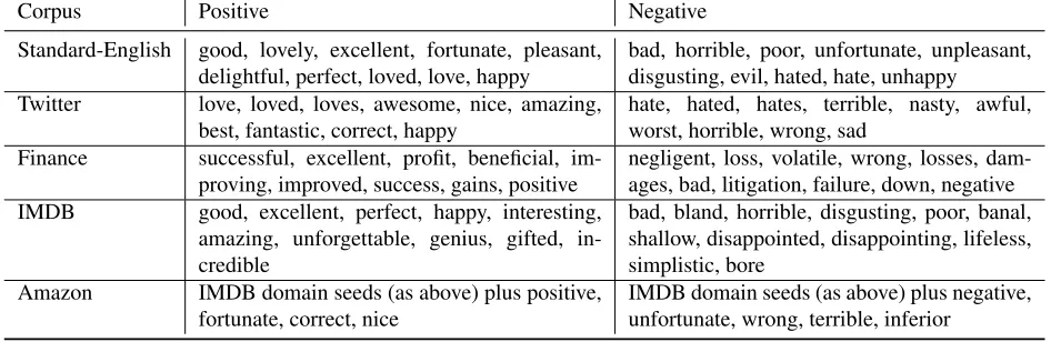
Table 1 shows the seed words for five different do-mains which areidenticalto those used by Hamilton et al. (2016) except for the two additional domains IMDB and Amazon. The induction of a sentiment lexicon could then be formulated as a simpleword
sentiment classification problem with two classes
(positive vs. negative). Each word is represented as a vector via domain-specific word embedding; the seed words are labeled with their correspond-ing classes while all the other words (i.e., “candi-dates”) are unlabeled; the task here is to learn a clas-sifier from the labeled examples first and then apply it to predict the sentiment polarity of each unlabeled candidate word. The probabilistic outputs of such a word sentiment classifier could be regarded as the measure of confidence about the predicted sentiment polarity. In the end, those candidate words with a high probability of being either positive or negative would be added to the sentiment lexicon. The final induced sentiment lexicon would include both the seed words and the selected candidate words.
As pointed out by Mudinas et al. (2012), if we simply consider all words from the given corpus as candidate words, the above described word senti-ment classifier tends to assign sentisenti-ment values not only to the actual sentiment words but also to their associated product features or more generally the
as-pectsof the expressed view. For example, if a lot of
customers do not like the weight of a product, the word sentiment classifier may assign strong nega-tive sentiment to “weight”, yet this is not stable — the sentiment polarity of “weight” may be different when a new version of the product is released or the
customer population has changed, and furthermore it probably does not apply to other products. To avoid this potential issue, it would be necessary to consider only a high-quality list of candidate words which are likely to be genuine sentiment words. Such a list of candidate words could be obtained directly from general-purpose sentiment lexicons. It is also possi-ble to perform NLP on the target domain corpus and extract frequently-occurring adjectives or other typi-cal sentiment indicators like emoticons as candidate words, which is beyond the scope of this paper.
To examine the effectiveness of different ma-chine learning algorithms for building such domain-specific word sentiment classifiers, we attempt to recreate known sentiment lexicons in three domains: Standard-English, Twitter, and Finance (see Sec-tion 3), in the same way as Hamilton et al. (2016) did. Put differently, for the purpose of evaluation, we would just use a known sentiment lexicon in the corresponding domain as the list of candidate words and see how different machine learning algorithms would classify those candidate words based on their domain-specific word embeddings. For those lexi-cons with ternary sentiment classification (positive vs. neutral vs. negative), the class-mass normal-ization method (Zhu et al., 2003) used by Hamilton et al. (2016) has been applied here to identify the neutral category. The quality of each induced lex-icon for a specific domain is evaluated by compar-ing it with its correspondcompar-ing known lexicon as the ground-truth, according to the performance metrics which are the same as in (Hamilton et al., 2016): Area Under the Receiver-Operating-Characteristic (ROC) Curve (AU C) for the binary classifications (ignoring the neutral class, as is common in pre-vious work) and Kendall’s τ rank correlation co-efficient with continuous human-annotated polarity scores. Note that Kendall’sτ is not suitable for the Finance domain, as its known sentiment lexicon is only binary. Therefore, our experimental setting and performance measures are all identical to those of Hamilton et al. (2016), which ensures the validity of the empirical comparison between our approach and theirs.
induc-Corpus Positive Negative Standard-English good, lovely, excellent, fortunate, pleasant,
delightful, perfect, loved, love, happy bad, horrible, poor, unfortunate, unpleasant,disgusting, evil, hated, hate, unhappy Twitter love, loved, loves, awesome, nice, amazing,
best, fantastic, correct, happy hate, hated, hates, terrible, nasty, awful,worst, horrible, wrong, sad Finance successful, excellent, profit, beneficial,
im-proving, improved, success, gains, positive negligent, loss, volatile, wrong, losses, dam-ages, bad, litigation, failure, down, negative IMDB good, excellent, perfect, happy, interesting,
amazing, unforgettable, genius, gifted, in-credible
bad, bland, horrible, disgusting, poor, banal, shallow, disappointed, disappointing, lifeless, simplistic, bore
Amazon IMDB domain seeds (as above) plus positive,
[image:8.612.70.543.59.213.2]fortunate, correct, nice IMDB domain seeds (as above) plus negative,unfortunate, wrong, terrible, inferior
Table 1: The “seeds” for domain-specific sentiment lexicon induction.
tion:
• kNN —kNearest Neighbors (Hastie et al., 2009),
• LR — Logistic Regression (Hastie et al., 2009),
• SVMlin— Support Vector Machine with the lin-ear kernel (Joachims, 1998),
• SVMrbf— Support Vector Machine with the non-linear RBF kernel (Joachims, 1998),
• TSVM — Transductive Support Vector Machine
(Joachims, 1999),
• S3VM — Semi-Supervised Support Vector
Ma-chine (Gieseke et al., 2012),
• CPLE — Contrastive Pessimistic Likelihood Es-timation (Loog, 2016),
• SGT — Spectral Graph Transducer (Joachims,
2003),
• SentProp — a label propagation based
classifica-tion method proposed for the SocialSent system (Hamilton et al., 2016).
The suitable parameter values of the above learning algorithms (such as theC for SVM) are found via grid search with cross-validation, and the probabilis-tic outputs are given by Platt scaling (Platt, 2000) if they are not provided by the original learning algo-rithm.
The experimental results shown in Table 2 demonstrate that in almost every single domain, simple linear model based supervised learning al-gorithms (LR and SVMlin) can achieve the op-timal or near-opop-timal accuracy for the sentiment lexicon induction task, and they outperform the state-of-the-art sentiment lexicon induction method SentProp (Hamilton et al., 2016) by a large mar-gin. The performance improvements are
statisti-cally significant (p-value < 0.05) according to the
sign test. There does not seem to be any benefit of utilizing non-linear models (kNN and SVMrbf) or semi-supervised/transductive learning algorithms (TSVM, S3VM, CPLE, SGT, and SentProp). The qualitative analysis of the sentiment lexicons in-duced by different methods shows that they differ only on those borderline, ambiguous words (such as “soft”) residing in the noisy overlapping region between two clusters in the vector space (see Sec-tion 3). In particular, SentProp is based on label propagation over the lexical graph of words, so it could be easily misled by noisy borderline words when sentiment clusters have considerable over-lap with each other, kind of “over-fitting” (Bishop, 2006). Furthermore, according to our experiments on the same machine, those simple linear models are 70+ times faster than SentProp. The speed dif-ference is mainly due to the fact that supervised learning algorithms only need to train on a small number of labeled words (“seeds” in our context) while semi-supervised/transductive learning algo-rithms need to train on not only a small number of labeled words but also a large number of unlabeled words.
Corpus Supervised Semi-Supervised/Transductive
kNN LR SVMlin SVMrbf TSVM S3VM CPLE SGT SentProp
AU C
Standard-English 0.892 0.931 0.939 0.941 0.901 0.540 0.680 0.852 0.906 Twitter 0.849 0.900 0.895 0.895 0.770 0.521 0.651 0.725 0.860 Finance 0.711 0.944 0.942 0.932 0.665 0.561 0.836 0.725 0.916
[image:9.612.72.546.56.152.2]τ Standard-English 0.469 0.495Twitter 0.490 0.569 0.4980.548 0.4950.547 0.4870.522 0.0380.001 0.1620.211 0.4090.437 0.4400.500
[image:9.612.315.539.210.365.2]Table 2: Comparing the induced lexicons with their corresponding known lexicons (ground-truth) according to the ranking of sentiment words measured byAU Cand Kendall’sτ.
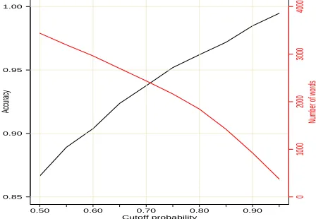
Fig. 5 shows that imposing a higher cut-off prob-ability threshold (for candidate words to enter the induced lexicon) would decrease the size of the in-duced lexicon but increase its quality (accuracy). On one hand, the induced lexicon needs to contain a suf-ficient number of sentiment words, especially when detecting sentiment from short texts, as a lexicon-based method cannot reasonably classify documents with none or too few sentiment words. On the other hand, the noise (misclassified sentiment words) in the induced lexicon would obviously have a detri-mental impact on the accuracy of the document sen-timent classifier built on top of it. Contrary to most previous work like that from Qiu et al. (2011) which tries to expand the sentiment lexicon as much as pos-sible and thus maintain a high recall, we would put more emphasis on the precision and keep a tight con-trol of the lexicon size. For us, having a small senti-ment lexicon is affordable, because our proposed ap-proach to document sentiment classification will be able to mitigate the low recall problem of lexicon-based methods by combining them with learning-based methods, which we shall talk about next.
5 Domain-Specific Sentiment Classification of Documents
A domain-specific sentiment lexicon, automatically induced using the above technique, provides a solid basis for building domain-specific document senti-ment classifiers. For the experisenti-ments here, we would use a list of 7866 candidate words constructed by merging two well-known general-purpose sentiment lexicons that are both publicly available — the ‘Gen-eral Inquirer’ (Stone et al., 1966) and the sentiment lexicon from Liu (2012). This set of candidate words is itself a combined, general-purpose sentiment
lex-Accuracy vs Size
0.85 0.90 0.95 1.00
Accur
acy
0
1000
2000
3000
4000
0.50 0.60 0.70 0.80 0.90
Cutoff probability
Number of words
Figure 5: How the accuracy and size of an in-duced lexicon are influenced by the cut-off proba-bility threshold.
icon, so we name it the GI+BL lexicon. Moreover, we would set the cut-off probability threshold to a generally good value 0.7 in our sentiment lexicon
induction algorithm. Comparing the IMDB vector space including all the candidate words (Fig. 4a) with that including only the high-probability candi-date words (Fig. 4b), it is obvious that the positive and negative sentiment clusters become more clearly separated in the latter.
detect the sentiment present in short texts, e.g., from Twitter, due to the lexical gap.
Given the induced sentiment lexicon, we propose to use a lexicon-based sentiment classifier to classify unlabeled documents, and then use those classified documents containing at least three sentiment words
aspseudo-labeleddocuments to be used later for the
training of a learning-based sentiment classifier. The condition of “at least three sentiment words” is to ensure that only reliably classified documents would be further utilised as training examples.
5.1 Sentiment Classification of Long Texts
First, we try the induced sentiment lexicons in the lexicon-based sentiment classifier pSenti (Mudinas et al., 2012) to see how good they are. Given a sen-timent lexicon, pSenti is able to perform not only binary sentiment classification but also ordinal sen-timent classification on a five-point scale. To mea-sure the binary classification performance, we use both micro-averagedF1(miF1) and macro-averaged
F1(maF1) which are commonly used in text
catego-rization (Yang and Liu, 1999). To measure the five-point scale classification performance, we use both Cohen’s κ coefficient (Manning et al., 2008) and also Root-Mean-Square Error (RM SE) (Bishop, 2006). As the baseline, we use a combined general-purpose sentiment lexicon, GI+BL, mentioned pre-viously in Section 4. As we can see from the results shown in Table 3, using the induced sentiment lex-icon for the target domain would make the lexlex-icon- lexicon-based sentiment classifier pSenti perform better than simply employing an existing general-purpose sen-timent lexicon. Moreover, using the sensen-timent lex-icons induced from the same domain would lead a much better performance than using the sentiment lexicons induced from a different domain.
Second, to evaluate the proposed two-phase boot-strapping method, we make empirical comparisons on the IMDB and Amazon datasets using a number of representative methods for document sentiment classification:
• pSenti — a concept-level lexicon-based sentiment classifier (Mudinas et al., 2012),
• ProbLex-DCM — a probabilistic lexicon-based classification using the Dirichlet Compound Multinomial (DCM) likelihood to reduce effective counts for repeated words (Eisenstein, 2017),
• SVMlin — Support Vector Machine with linear kernel (Joachims, 1998),
• CNN — Convolutional Neural Network (Kim,
2014),
• LSTM — Long Short-Term Memory, a Recurrent Neural Network (RNN) that can remember val-ues over arbitrary time intervals (Hochreiter and Schmidhuber, 1997; Dai and Le, 2015).
To apply the deep learning algorithms CNN and LSTMthathaveawordembeddingprojectionlayer, wefixthereviewsizeto500words,truncating re-viewslongerthanthatandpaddingreviews shorter thanthatwithnullvalues. As pointedoutbyGreff etal. (2017), the hiddenlayersize isan important hyperparameterofLSTM:usuallythelargerthe net-work,thebettertheperformancebutthelongerthe trainingtime. Inourexperiments,wehaveusedan LSTMnetwork with 400unitson thehiddenlayer whichisthecapacitythataPCwithoneNvidiaGTX 1080TiGPUcanaffordandadropout(Wageretal., 2013)rateof0.5whichisthemostcommonsetting inresearchliterature(Srivastava etal.,2014; Hong andFang,2015;Cliche,2017).
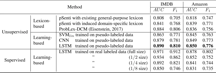
As shown in Table 4, the above described two-phasebootstrappingmethodhasbeendemonstrated tobebeneficial:thelearning-basedsentiment clas-sifierst rainedo np seudo-labeledd ataa re supe-riortolexicon-basedsentimentclassifiers,including thestate-of-the-artunsupervisedsentimentclassifier ProbLex-DCM(Eisenstein,2017).Furthermore,the two-phasebootstrappingmethodisageneral frame-workwhichcanutilizeanylexicon-basedsentiment classifiert op roducep seudo-labeledd ata. There-fore the more sophisticated ProbLex-DCM could also be used instead of pSenti in this framework, which is likely to deliver an even higher perfor-mance. Among thethree learning-basedsentiment classifiers,LSTMachievedthebestperformanceon bothdatasets,whichisconsistentwiththe observa-tionsinotherstudieslikeDaiandLe(2015).
ComparingtheLSTM-basedsentimentclassifiers trainedonpseudo-labeledandreallabeleddata,we can also see that using a large number of pseudo-labeled examples could achieve a similar effect as using 25/4 ≈ 6k and 8/2 = 4k real labeled
Lexicon miF binary 5-point scale
1 maF1 F1pos F1neg Cohen’sκ RM SE
general-purpose GI+BL 0.745 0.744 0.764 0.722 0.235 1.325
[image:11.612.81.531.57.139.2]domain-specific same domain (Kitchen)different domain (Electronics) 0.7490.761 0.761 0.772 0.7500.749 0.750 0.749 0.2360.215 1.3101.373 different domain (Video) 0.736 0.735 0.752 0.717 0.206 1.372
Table 3: Lexicon-based sentiment classification of Amazon Kitchen product reviews.
Method AU CIMDBF Amazon
1 AU C F1
Unsupervised
Lexicon-based
pSenti with existing general-purpose lexicon 0.808 0.705 0.818 0.747 pSenti with induced domain-specific lexicon 0.841 0.768 0.839 0.771 ProbLex-DCM (Eisenstein, 2017) 0.884 0.806 0.836 0.756
Learning-based
SVMlintrained on pseudo-labeled data 0.863 0.771 0.845 0.763
CNN trained on pseudo-labeled data 0.879 0.781 0.849 0.773 LSTM trained on pseudo-labeled data 0.890 0.810 0.850 0.776
Supervised Learning-based
LSTM trained on real labeled data (full size) 0.971 0.912 0.878 0.802 ” (1/2size) 0.934 0.862 0.852 0.752 ” (1/4size) 0.892 0.821 0.841 0.744 ” (1/8size) 0.850 0.746 0.831 0.735
Table 4: Sentiment classification of long texts.
only a few thousand (or less) labeled examples.
5.2 Sentiment Classification of Short Texts
To evaluate our proposed approach to sentiment classification of short texts, we have carried out experiments on the Twitter sentiment classification benchmark dataset from SemEval-2017 Task 4B (Rosenthal et al., 2017) which is to classify 6185
tweets as either positive or negative. Other than the training set of20,508tweets, we also collected
un-labeled tweets using the Twitter API. All the tweets would be pre-processed by replacing emoticons with their corresponding text representations and encod-ing URLs by tokens. In addition to the Twitter-domain seed words listed in Table 1, we have also made use of common positive/negative emoticons which are ubiquitous on Twitter as additional seeds for the task of sentiment lexicon induction. Note that in all our experiments, we do not use the sen-timent labels and the topic information provided in the training data.
Making use of the provided training data and our own unlabeled data collected from Twitter, we have constructed the domain-specific word embeddings,
induced the sentiment lexicon, and bootstrapped the pseudo-labeled tweet data to train the binary tweet sentiment classifier. As the learning algorithm we have chosen LSTM with a hidden layer of 150 units which would be enough for tweets as they are quite short (with an average length of only 20 words).
The official performance measures for this short text sentiment classification task (Rosenthal et al., 2017) include Accuracy (Acc) and F1. Although
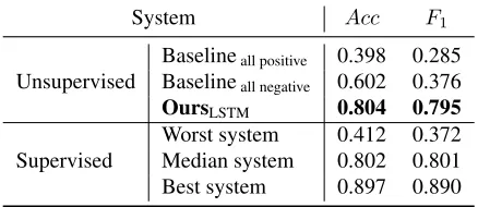
our approach is nearly-unsupervised (without any reliance on labeled documents), its performance on this benchmark dataset is comparable to that of su-pervised methods: it would be placed roughly in the middle of all the participating systems in this com-petition (see Table 5).
5.3 Detecting Neutral Sentiment
[image:11.612.78.536.175.331.2]System Acc F1
Unsupervised BaselineBaselineall positiveall negative 0.398 0.2850.602 0.376
OursLSTM 0.804 0.795
[image:12.612.76.295.56.151.2]Supervised Worst systemMedian system 0.412 0.3720.802 0.801 Best system 0.897 0.890
Table 5: Sentiment classification of short texts into two categories — SemEval-2017 Task 4B.
to recognize neutral sentiment is challenging. To investigate this issue, we have done experiments on the Twitter sentiment classification benchmark dataset from SemEval-2017 Task 4C (Rosenthal et al., 2017) which is to classify12379tweets into an
ordinal five-point scale (−2,−1,0,+1,+2) where 0represents the neutral class.
One common way to handle neutral sentiment is to treat the set of neutral documents as a sepa-rate class for the classification algorithm, which is the method advocated by Koppel and Schler (2006). With the pseudo-labeled training examples of three classes (−1: negative, 0: neutral, and +1:
posi-tive), we tried both standard multi-class classifica-tion (Hsu and Lin, 2002) and ordinal classificaclassifica-tion (Frank and Hall, 2001). However, neither of them could deliver a reasonable performance. After care-fully inspecting the classification results, we realised that it is very difficult to have a set of representative training examples with good coverage for the neu-tral class. This is because the neuneu-tral class is not homogeneous: a document could be neutral because it is equally positive and negative, or because it does not contain any sentiment. In practice, the latter case is more often seen than the former case, and it im-plies that the neutral class is more often defined by the absence of sentiment word features rather than their presence, which would be problematic to most supervised learning algorithms.
What we discovered is that the simple method of identifying neutral documents from the binary sentiment classifier’s decision boundary works sur-prisingly well, as long as the right thresholds are found. Specifically, we take the probabilistic out-puts of a binary sentiment classifier trained as be-fore, and then put all the documents whose
proba-bility of being positive lies not close to 0, not close to 1, but in the middle range into the neutral class. It turns out thatprobability calibration (Niculescu-Mizil and Caruana, 2005) is crucially important for this simple method to work. Some supervised learn-ing algorithms for classification can give poor es-timates of the class probabilities, and some even do not support probability prediction. For instance, maximum-margin learning algorithms such as SVM focus on hard samples that are close to the deci-sion boundary (the support vectors), which makes their probability prediction biased. The technique of probability calibration allows us to better calibrate the probabilities of a given classifier, or to add sup-port for probability prediction. If a classifier is well calibrated, its probabilistic output should be able to be directly interpreted as a confidence level on the prediction. For example, among the documents to which such a calibrated binary classifier gives a probabilistic output close to0.8, approximately 80%
of the documents would actually belong to the posi-tive class.
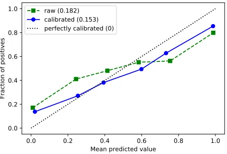
Using the sigmoid model of Platt (2000) with cross-validation on the pseudo-labeled training data, we carry out probability calibration for our LSTM based binary sentiment classifier. Fig. 6 shows that the calibrated probability prediction aligns with the true confidence of prediction much better than the raw probability prediction. In this case, the Brier loss (Brier, 1950) that measures the mean squared difference between the predicted probability and the actual outcome could be reduced from 0.182 to 0.153 by probability calibration.
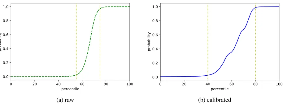
If we rank the estimated probabilities of being positive from low to high, the curve of probabili-ties would be in an “S”-shape with a distinct middle range where the slope is steeper than the two ends, as shown in Fig. 7. The documents with their probabil-ities of being positive in such a middle range should be neutral. Therefore the two elbow points in the probability curve would make appropriate thresh-olds for the identification of neutral sentiment, and they could be found automatically by a simple algo-rithm using the central difference to approximate the second derivative. LetpL andpU denote the identi-fied thresholds (pL< pU), then we assign class label “−1” to all those documents with the probability
proba-System M AEµ M AEM miF1 maF1
Unsupervised
Baselineall -2 1.895 2.000 0.006 0.014
Baselineall -1 0.923 1.400 0.089 0.286
Baselineall 0 0.525 1.200 0.133 0.500
Baselineall +1 1.127 1.400 0.063 0.188
Baselineall +2 2.105 2.000 0.004 0.011
Lexicon-based 0.939 1.135 0.253 0.189
OursLSTM 0.536 0.815 0.537 0.326
[image:13.612.155.458.55.199.2]Supervised Worst systemMedian system 0.9850.509 1.3250.823 0.2500.545 0.1210.299 Best system 0.554 0.481 0.504 0.405
Table 6: Sentiment classification of short texts on a five-point scale — SemEval-2017 Task 4C.
0.0 0.2 0.4 0.6 0.8 1.0
Mean predicted value 0.0
0.2 0.4 0.6 0.8 1.0
Fraction of positives
raw (0.182) calibrated (0.153) perfectly calibrated (0)
Figure 6: The probability calibration plot of our LSTM-based sentiment classifier on the SemEval-2017 Task 4C dataset.
bility abovepU, and “0” to all those documents with the probability within[pL, pU].
The official performance measures for this sen-timent classification task (Rosenthal et al., 2017) are M AEµ and M AEM which stand for micro-averaged and macro-micro-averaged Mean Absolute Er-ror (MAE), respectively. We would also like to report the micro-averaged and macro-averaged F1
scores which are denoted as miF1and maF1
respec-tively. As shown in Fig. 7, the thresholds identi-fied from the raw probability curve are roughly at 55 percentile and 75 percentile, which would yield M AEµ= 0.632andM AEM = 0.832; the
thresh-olds identified from the calibrated probability curve are roughly at 40 percentile and 80 percentile, which would yield much better scores M AEµ = 0.536
andM AEM = 0.815. So with the help of
probabil-ity calibration, our proposed approach would be able to comfortably beat all the baselines including the lexicon-based method pSenti (Mudinas et al., 2012) and compete with the average (median) participat-ing systems (see Table 6). Please note that this is not a fair comparison: our approach is at a great disadvantage because (i) it is nearly-unsupervised, without any reliance on labeled documents while all the other systems are supervised; and (ii) it performs only ternary classification while all the other sys-tems make classification on the full five-point scale.
6 Conclusions
How far can we go in sentiment classification for a new domain, given only unlabeled data? This pa-per presents our exploration towards answering the above research question. Specifically, the main con-tributions of this paper are as follows.
• We have formulated the cluster hypothesis for sentiment analysis (i.e., words with different sen-timent polarities form distinct clusters) and veri-fied that in general it holds for word embeddings within a specific domain but not across domains.
[image:13.612.74.299.245.398.2]0 20 40 60 80 100 percentile
0.0 0.2 0.4 0.6 0.8 1.0
probability
(a) raw
0 20 40 60 80 100
percentile 0.0
0.2 0.4 0.6 0.8 1.0
probability
[image:14.612.80.537.54.224.2](b) calibrated
Figure 7: The probability curve with a region of intermediate probabilities representing the neutral class.
our system clearly outperforms the state-of-the-art sentiment lexicon induction method — Sent-Prop (Hamilton et al., 2016).
• We have shown that a lexicon-based sentiment classifier could be enhanced by using its out-puts as pseudo-labels and employing supervised learning algorithms such as LSTM to train a learning-based sentiment classifier on pseudo-labeled documents. Our end-to-end pipelined ap-proach which, overall, is unsupervised (except for a very small set of seed words), works bet-ter than the state-of-the-art unsupervised tech-nique for document sentiment classification — ProbLex-DCM (Eisenstein, 2017), and its perfor-mance is at least on par with an average fully supervised sentiment classifier trained on real la-beled data (Rosenthal et al., 2017).
• We have revealed the crucial importance of prob-ability calibration to the detection of neutral sen-timent which was overlooked in previous studies (Koppel and Schler, 2006). With the right thresh-olds found, neutral documents can be simply iden-tified at the binary sentiment classifier’s decision boundary.
One promising way to further enhance the LSTM-based sentiment classifier in the proposed approach with the induced sentiment lexicon would be to con-catenate word embeddings with an indicator feature which tells whether a current word is positive, neu-tral, or negative (Ebert et al., 2015). We leave this for future work.
Acknowledgements
The Titan X Pascal GPU used for this research was kindly donated by the NVIDIA Corporation. We thank the reviewers for their constructive and help-ful comments. We also gratehelp-fully acknowledge the support of Geek.AI for this work.
References
Shlomo Argamon, Casey Whitelaw, Paul J. Chase, Sob-han Raj Hota, Navendu Garg, and Shlomo Levitan. 2007. Stylistic text classification using functional lexi-cal features. Journal of the American Society for Infor-mation Science and Technology (JASIST), 58(6):802– 822.
Christopher M. Bishop. 2006. Pattern Recognition and Machine Learning. Springer-Verlag.
John Blitzer, Mark Dredze, and Fernando Pereira. 2007. Biographies, bollywood, boom-boxes and blenders: Domain adaptation for sentiment classification. In
Proceedings of the 45th Annual Meeting of the As-sociation for Computational Linguistics (ACL), pages 440––447, Prague, Czech Republic.
Danushka Bollegala, David J. Weir, and John A. Car-roll. 2013. Cross-domain sentiment classification us-ing a sentiment sensitive thesaurus. IEEE Transac-tions on Knowledge and Data Engineering (TKDE), 25(8):1719–1731.
Johan Bollen, Huina Mao, and Xiao-Jun Zeng. 2011. Twitter mood predicts the stock market. Journal of Computational Science, 2(1):1–8.
Mathieu Cliche. 2017. BB twtr at SemEval-2017 Task 4: Twitter sentiment analysis with CNNs and LSTMs. In
Proceedings of the 11th International Workshop on Se-mantic Evaluation (SemEval@ACL 2017), pages 573– 580, Vancouver, Canada.
Andrew M. Dai and Quoc V. Le. 2015. Semi-supervised sequence learning. InAdvances in Neural Information Processing Systems 28: Annual Conference on Neural Information Processing Systems (NIPS), pages 3079– 3087, Montreal, Canada.
Xiaowen Ding, Bing Liu, and Philip S. Yu. 2008. A holistic lexicon-based approach to opinion mining. In
Proceedings of the International Conference on Web Search and Web Data Mining (WSDM), pages 231– 240, Palo Alto, CA, USA.
Sebastian Ebert, Ngoc Thang Vu, and Hinrich Sch¨utze. 2015. A linguistically informed convolutional neu-ral network. InProceedings of the 6th Workshop on Computational Approaches to Subjectivity, Sentiment and Social Media Analysis (WASSA@EMNLP), pages 109–114, Lisbon, Portugal.
Jacob Eisenstein. 2017. Unsupervised learning for lexicon-based classification. In Proceedings of the 31st AAAI Conference on Artificial Intelligence (AAAI), pages 3188–3194, San Francisco, CA, USA. Ethan Fast, Binbin Chen, and Michael S. Bernstein.
2016. Empath: Understanding topic signals in large-scale text. InProceedings of the 2016 CHI Conference on Human Factors in Computing Systems (CHI), pages 4647–4657, San Jose, CA, USA.
Eibe Frank and Mark A. Hall. 2001. A simple approach to ordinal classification. In Proceedings of the 12th European Conference on Machine Learning (ECML), pages 145–156, Freiburg, Germany.
Fabian Gieseke, Antti Airola, Tapio Pahikkala, and Oliver Kramer. 2012. Sparse quasi-Newton opti-mization for semi-supervised support vector machines. In Proceedings of the 1st International Conference on Pattern Recognition Applications and Methods (ICPRAM), pages 45–54, Vilamoura, Algarve, Portu-gal.
Xavier Glorot, Antoine Bordes, and Yoshua Bengio. 2011. Domain adaptation for large-scale sentiment classification: A deep learning approach. In Pro-ceedings of the 28th International Conference on Ma-chine Learning (ICML), pages 513–520, Bellevue, WA, USA.
Yoav Goldberg. 2017. Neural network methods for natu-ral language processing.Synthesis Lectures on Human Language Technologies, 10(1):1–309.
Klaus Greff, Rupesh Kumar Srivastava, Jan Koutn´ık, Bas R. Steunebrink, and J¨urgen Schmidhuber. 2017. LSTM: A search space odyssey. IEEE Transactions
on Neural Networks and Learning Systems (TNNLS), 28(10):2222–2232.
William L. Hamilton, Kevin Clark, Jure Leskovec, and Dan Jurafsky. 2016. Inducing domain-specific senti-ment lexicons from unlabeled corpora. InProceedings of the 2016 Conference on Empirical Methods in Nat-ural Language Processing (EMNLP), pages 595–605, Austin, TX, USA.
Trevor Hastie, Robert Tibshirani, and Jerome Friedman. 2009. The Elements of Statistical Learning: Data Mining, Inference, and Prediction. Springer, 2nd edi-tion.
Sepp Hochreiter and J¨urgen Schmidhuber. 1997. Long short-term memory. Neural Computation, 9(8):1735– 1780.
James Hong and Michael Fang. 2015. Sentiment anal-ysis with deeply learned distributed representations of variable length texts. Technical report, Stanford Uni-versity.
Chih-Wei Hsu and Chih-Jen Lin. 2002. A comparison of methods for multiclass support vector machines. IEEE Transactions on Neural Networks (TNN), 13(2):415– 425.
Minqing Hu and Bing Liu. 2004. Mining and summa-rizing customer reviews. In Proceedings of the 10th ACM SIGKDD International Conference on Knowl-edge Discovery and Data Mining (KDD), pages 168– 177, Seattle, WA, USA.
Yohan Jo and Alice H. Oh. 2011. Aspect and sentiment unification model for online review analysis. In Pro-ceedings of the 4th International Conference on Web Search and Web Data Mining (WSDM), pages 815– 824, Hong Kong, China.
Thorsten Joachims. 1998. Text categorization with sup-port vector machines: Learning with many relevant features. InProceedings of the 10th European Confer-ence on Machine Learning (ECML), pages 137–142, Chemnitz, Germany.
Thorsten Joachims. 1999. Transductive inference for text classification using support vector machines. In
Proceedings of the 16th International Conference on Machine Learning (ICML), pages 200–209, Bled, Slovenia.
Thorsten Joachims. 2003. Transductive learning via spectral graph partitioning. In Proceedings of the 20th International Conference on Machine Learning (ICML), pages 290–297, Washington, DC, USA. Yoon Kim. 2014. Convolutional neural networks for
sen-tence classification. InProceedings of the 2014 Con-ference on Empirical Methods in Natural Language Processing (EMNLP), pages 1746–1751, Doha, Qatar. Moshe Koppel and Jonathan Schler. 2006. The im-portance of neutral examples for learning sentiment.