HOG ACTIVE APPEARANCE MODELS
Epameinondas Antonakos
?, Joan Alabort-i-Medina
?, Georgios Tzimiropoulos
†?, Stefanos Zafeiriou
? ?Imperial College London, Department of Computing, U.K.
†
University of Lincoln, School of Computer Science, U.K.
ABSTRACT
We propose the combination of dense Histogram of Oriented Gradi-ents (HOG) features with Active Appearance Models (AAMs). We employ the efficient Inverse Compositional optimization technique and show results for the task of face fitting. By taking advantage of the descriptive characteristics of HOG features, we build robust and accurate AAMs that generalize well to unseen faces with illu-mination, identity, pose and occlusion variations. Our experiments on challenging in-the-wild databases show that HOG AAMs signif-icantly outperfrom current state-of-the-art results of discriminative methods trained on larger databases.
Index Terms— Active Appearance Models, Histogram of Ori-ented Gradients, Inverse Compositional optizimation
1. INTRODUCTION
Active Appearance Models (AAMs) are generative parametric de-formable statistical models of the shape and appearance variation of an object that are widely used in various tasks of Human-Computer Interaction and Image and Video Processing. They have been used in numerous applications such as face fitting, facial expressions recog-nition and medical imaging. They were initially proposed in [1] and they are descendants of Active Contour Models [2] and Active Shape Models [3]. The fitting process of an AAM aims to bring a test im-age into registration with a reference template, even if the test imim-age is a deformed instance of the template. The most common choise for fitting an AAM is the Inverse Compositional (IC) optimization techique [4, 5, 6], though other methodologies have been used, such as regression [1, 7]. IC is a non-linear gradient descent optimiza-tion algorithm that attempts to minimize the discrepancy between a warped input image and a parametric model instance with respect to the shape and appearance parameters.
Since IC is a gradient descent method, the alignment is sensitive to initialization and to large appearance variations in terms of illumi-nation, expressions, occlusion and identity. Especially, in the case of intensities-based AAMs with the Project-Out IC algorithm [4], the model is incapable of adequately generalizing in order to be robust to outliers. This is the main reason why AAMs have been criticized of being able to perform well only in person specific applications and not generic ones. In this paper, we show that the combination of the IC framework with a powerful and descriptive features descriptor results in a generic deformable model with remarkable performance. The concept of dense feature-based image representation is also adopted in [8], where the authors use correspondences be-tween densely computed SIFT descriptors. However it is applied
The work of Epameinondas Antonakos and Stefanos Zafeiriou was par-tially funded by the EPSRC project EP/J017787/1 (4D-FAB). The work of Joan Alabort-i-Medina was funded by the Qualcomm Innovation Fellowship and by a European DTA from Imperial College London.
on scene alignment and face recognition and not on deformable models fitting. There are several attempts in recent bibliography to build a feature-based AAM framework. The authors in [9] use novel features based on the orientations of gradients to represent edge structure within a regression framework. Similar features are employed in [6] to create a robust similarity optimization criterion. In [10] a combination of grayscale intensities, hue channel and edge magnitude is used to build the appearance model. Moreover, the work in [11] applies the IC optimization algorithm in the Fourier domain using Gabor responses. In [12] a new appearance repre-sentation is introduced for AAMs by combining Gabor wavelet and Local Binary Pattern descriptor. The authors in [13] employ Gabor magnitude features summed over either orientations or scales or both to build an appearance model. Similarly, the authors in [14] model the characteristic functions of Gabor magnitude and phase by using lognormal and Gaussian density functions respectively and utilize the mean of the characteristics over orientations and scales.
In this paper, we employ densely-sampled Histogram of Ori-ented Gradients (HOG) features [15] to train the AAM appearance model. To the best of our knowledge, this is the first time that a generic feature-based AAM is developped using dense HOGs. We perform cross-database experiments on in-the-wild images us-ing two IC algorithms: Alternatus-ing IC (AIC) [5] and Project-Out IC (POIC) [4]. Finally, we show that our HOG AAMs greatly outperform state-of-the-art methods in facial alignment, which are discriminatively trained on much more data than our approach.
2. HISTOGRAMS OF ORIENTED GRADIENTS
We extractdenseHOG descriptors at each pixel of an image, based on the method introduced in [15]. This means that given an input image of sizeH ×W, the densely-sampled multichannel features image has sizeH×W×D. Let us denote the HOG features ex-traction function asHand an input image in vectorial form astwith lengthLT. Then the HOG image in vectorial form is
h=H(t) (1)
whereH : RLT×1 −→ RLTD×1. The HOG extraction func-tion clusters gradient orientafunc-tions in different bins for localized sub-windows of the input image. Specifically, we first compute the im-age gradient and in the case of an RGB imim-age, we keep the gradient with the largest norm between the gradients of the three channels. For each pixel of the image, we use two spatial neighbourhoods: cells and blocks. Acellis a small rectangular sub-window of size
Ncellpixels in height and width, from which we create a histogram
of the gradient orientations weighted by the gradient magnitude of each pixel. This orientation binning procedure reveals the non-linear nature of the HOG descriptors. Each histogram hasNbinsand we
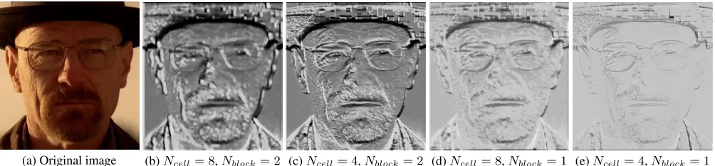
(a) Original image (b)Ncell= 8,Nblock= 2 (c)Ncell= 4,Nblock= 2 (d)Ncell= 8,Nblock= 1 (e)Ncell= 4,Nblock= 1
Fig. 1. Example of dense HOG features.Ncelldenotes the cell height and width in pixels andNblockdenotes the number of cells that consist
a block. Thus,(b)and(c)haveD= 36channels whereas(d)and(f)haveD= 9channels. We visualize the sum over all theDchannels.
centres with respect to orientation and position. Ablockis a larger spatial neighbourhood that consists ofNblock×Nblockcells. After
applying contrast normalization at each block, the final descriptor vector at each image pixel is constructed by concatenating the his-tograms of the cells, thus it has lengthD=NbinsNblock2 .
The local contrast normalization adopted at each block is es-sential as it makes the features image invariant to illumination and foreground-background intense differences. Thus, HOG features have great advantages, such as invariance to geometric and photo-metric variations, which are important for building robust generic deformable models. We altered the code provided by [16] in order to extract dense HOG features. We useNbins = 9histogram bins
and experiment with the cell size (Ncell ∈ {4,8}) and the block
normalization (Nblock ∈ {1,2}). Figure 1 shows indicative HOG
images by summing over all their channels.
3. HOG ACTIVE APPEARANCE MODELS
3.1. Training
Let us denote a shape instance of LS landmark points as s =
[x1, y1, . . . , xLS, yLS] T
. Theshape modelis constructed by align-ing a set of trainalign-ing shapes {si} using Genaralized Procrustes
Analysis and applying Principal Component Analysis (PCA) on the aligned shapes to end up with an orthonormal basis ofNS
eigen-vectorsUS ∈ R2LS×NS and the mean shape ¯s. The first four
eigenshapes correspond to the similarity transform parameters that control the global rotation, scaling and translation. A shape instance is generated assp = ¯s+USp, wherepis theNS×1vector of
shape parameters. Themotion modelconsists of the warp function
W(p), which maps the points within a source shape to their corre-sponding coordinates in a target shape. We employ the Piecewise Affine Warp, which performs the mapping based on the barycentric coordinates of the corresponding triangles between the two shapes that are extracted using Delaunay Triangulation.
Given a set of training annotated images{ti}, we compute their
HOG features{hi}(Eq. 1) and warp them into the mean shape¯s,
ending up with a set of aligned vectors. Each vector has length
LA, i.e. the number of pixels that lay inside the mean shape. Then
we apply PCA to find an appearance subspaceUA ∈ RLA×NA ofNA eigentextures and the mean appearance vector ¯a.
Synthe-sis is achieved through linear combination of the eigentextures as
aλ = ¯a+UAλ, whereλis theNA×1appearance parameters
vector.
3.2. Inverse Compositional Optimization
The aim of AAM fitting is to minimize the`2-norm between an
in-put vectorized HOG imagehand the HOG appearance model with respect to the shape and appearance parameters, i.e.
argminp,λkh(W(p))−¯a−UAλk2 (2)
In general, the IC optimization introduces an incremental warp that is applied on the residual term as
argmin∆p,λkh(W(p))−¯a(W(∆p))−UA(W(∆p))λk2
This problem is solved by performing a first order Taylor expansion on the residual term with respect to the parameters increment∆p
and composing the current warp with the incremental warp at each iteration asW(p)← W(p)◦ W(∆p)−1. The linearization is
¯
a(W(∆p)) +UA(W(∆p))λ≈¯a+UAλ+J|p=0∆p
whereJ|p=0 =∇(¯a+UAλ) ∂∂Wp
p=0is the Jacobian. Note that the appearance model is based on the HOG representation of Eq. 1. Hence, in the partial derivative of the Jacobian, we make the assump-tion that∂∂Ht∇t≈ ∇H(t), which means that we neglect the partial derivative ofHand deal withH(t)as a multichannel image. In this work, we use the Alternating and Project-Out IC algorithms.
Alternating:The AIC algorithm, proposed in [5], deals with the problem of Eq. 2, by solving two separate minimization problems, one for the shape and one for the appearance optimal parameters, in an alternating manner. The two cost functions are
(
argmin∆pkh(W(p))−aλ(W(∆p))k2I−UAUTA
argmin∆λkh(W(p))−aλ+∆λ(W(∆p))k2
(3)
The minimization in every iteration is achieved by first using a fixed estimate ofλto compute the current estimate of∆pand then us-ing the fixed estimate ofpto compute the increment∆λ. More specifically, given the current estimate ofλ, the shape parameters increment is computed from the first cost function using the orthog-onal complement of the appearance subspaceUˆA = I−UAUTA
as
∆p=H−1JTAIC[h(W(p))−a¯−UAλ]
where JAIC = UˆA[J¯a|p=0 +PiN=1AλiJui|p=0] and H
−1
=
JT
AICJAIC. Then, given the current estimate of the parameters p, AIC computes the optimal appearance parameters as the least-squares solution of the second cost function of Eq. 3, thus
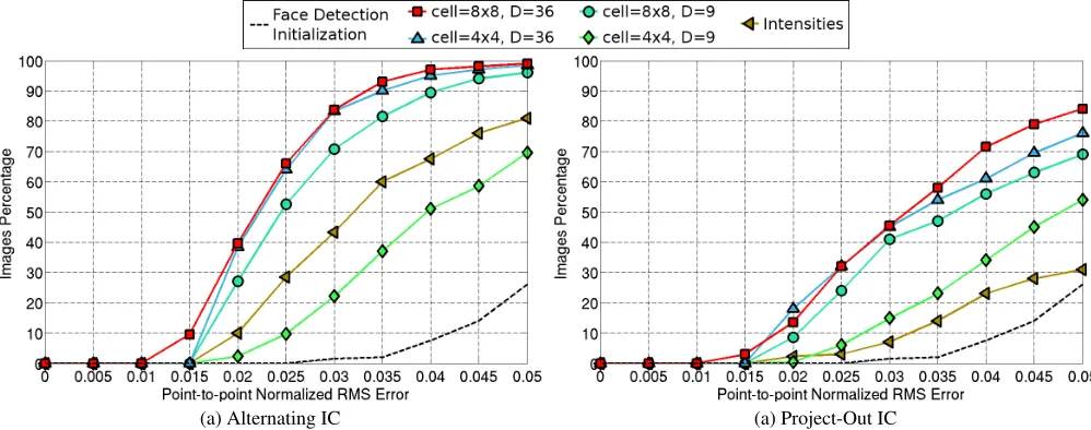
[image:2.612.55.557.71.188.2](a) Alternating IC (a) Project-Out IC
Fig. 2. Experimental results on the LFPW testing database evaluated on 68 points mask. We use various values for the HOG parameters (Ncell∈ {4,8},Nblock∈ {1,2}) and also compare with the intenisities-based AAMs using both the Alternating and Project-Out algorithms.
This alternating optimization is repeated at each iteration. The ap-pearance parameters are updated in an additive mode, i.e.λ←λ+ ∆λ. Although the individual JacobiansJui|p=0, ∀i= 1, . . . , NA
andJ¯a|p=0can be precomputed, the total JacobianJAIC and the
Hessian need to be evaluated at each iteration. Following the Hes-sian matrix computation technique proposed in [5], which improves the cost fromO(NS2LA)toO(NS2N
2
A) (usuallyLA > NA2), the
total cost at each iteration isO(N2
SNA2+ (NS+NA)LA+NS3). Project-Out:The POIC algorithm [4] decouples shape and ap-pearance by solving Eq. 2 in the subspace that is orthogonal to the appearance variation. This is achieved by “projecting-out” the ap-pearance variation, thus, similar to the first problem of Eq. 3, the solution is computed based on the orthogonal complement of the ap-pearance subspaceUˆA=I−UAUTA. The difference with the AIC
case is that there is not an extra step for optimizing with respect to the appearance parameters. The cost function of Eq. 2 takes the form
argmin∆pkh(W(p))−a¯(W(∆p))k
2
I−UAUTA (4)
and the first-order Taylor expansion is¯a(W(∆p))≈a¯+J¯a|p=0∆p. The shape parameters increment is computed as
∆p=H−1JTP OIC[h(W(p))−a¯]
whereH−1 =JTP OICJP OICandJP OIC= ˆUAJ¯a|p=0. The ap-pearance parameters can be retrieved at the end of the iterative oper-ation asλ=UT
A[h(W(p))−¯a]in order to reconstruct the
appear-ance vector. The POIC algorithm is faster than AIC, with compu-tational complexity ofO(NSLA+NS2), because the Jacobian, the
Hessian matrix and its inverse are constant and can be precomputed.
4. EXPERIMENTAL RESULTS
In this section we carry out experiments on three challenging in-the-wild databases, which consist of images downloaded from the web that are captured in totally unconstrained conditions and exhibit large variations in pose, identity, illumination, expressions, occlu-sion and resolution. We train our HOG-AAM model on 811 training images of the LFPW [17] training set (the rest of the database’s im-ages URLs are invalid), keepingNS = 15eigenshapes andNA =
100eigentextures. We acquired the groundtruth annotations of 68 points from the 300 Faces In-The-Wild Challenge [18]. The fit-ting process is initialized by compufit-ting the face’s bounding box using the Cascade Deformable Part Models face detector [19] and then estimating the appropriate global similarity transform that fits the mean shape within the bounding box bounds. Note that this initial similarity transform only involves a translation and scaling component and not any in-plane rotation. The accuracy of the fit-ting results is measured by the point-to-point RMS error normalized by the face size, as proposed in [20]. Denoting the fitted and the groundtruth shapes assf
andsg
respectively and the face’s size as
sf = (maxxgi −minx g
i + maxy g
i −miny g
i)/2, then the error is
expressed as RMSE=
PL i=1
q
(xfi−xgi)2+(yfi−ygi)2
sfLS .
Comparison between HOG Features Variants: Herein, we conduct an experiment to compare the performance of HOG AAMs for various combinations of the parameters values presented in Sec. 2. Specifically, we use cell size values ofNcell ∈ {4,8}and
experiment with the employment of block normalization by setting
Nblock ∈ {1,2}, which results in HOG images withD ∈ {9,36}
number of channels. Moreover, we compare our HOG AAMs with the intensities-based AAMs. The experiment is performed on the 224 images of the LFPW testing set. The results are demonstrated in Fig. 2 in the form of Cumulative Error Distribution (CED). This experiment proves that the block normalization has a great impact on the fitting result, while the reduction of the cell size provokes a small decline on the fitting accuracy. Additionally, HOG AAMs clearly outperform the intensities-based AAMs. Especially, in the case of HOGs wichNcell = 8and block normalization (D = 36),
the difference is approximately 30% and 40% in the cases of RMSE less than 0.02 and 0.03 respectively.
[image:3.612.57.556.72.269.2](a) Helen Database (a) AFW Database
Fig. 3. Comparison of HOG AAMs with state-of-the-art methods (SDM [7], DRMF [21]) on Helen and AFW databases, evaluated on 49 points mask.
Fig. 4. Fitting examples using HOG-AIC on AFW and Helen images.Top row:Initialization from bounding box.Bottom row:Fitting result.
Method Helen AFW
mean std mean std
HOG-AIC 0.0184 0.0058 0.0215 0.0129
[image:4.612.56.559.70.268.2]SDM 0.0216 0.0059 0.0484 0.5002 HOG-POIC 0.0300 0.0140 0.0395 0.0212 DRMF 0.0280 0.0086 0.0517 0.0611 Face Detection 0.0532 0.0196 0.0635 0.0227
Table 1. Statistics (mean and standard deviation) of Figure 3 results.
We use the best performing HOG parameters from the previous ex-periment, thus we set the cell size at8×8pixels and the block size at2×2cells, ending up with HOG feature images ofD= 36 chan-nels. The testing is performed on the very challenging in-the-wild databases of AFW [20] and Helen [22] which consist of 337 and 330 testing images respectively. Similar to the LFPW database, we acquired the groundtruth annotations from [18]. In this experiment we report results evaluated on 49 points shape mask instead of the 68 points of the previous one. This is because the SDM framework [7] returns only these 49 points, which occur by removing the 17 points of the boundary (jaw) and the 2 points from the mouth’s corners. Thus, this evaluation framework emphasizes on the internal facial areas (eyebrows, eyes, nose, mouth).
Figure 3 demonstrates the results on Helen and AFW databases and Table 1 reports the corresponding statistics (mean and standard deviation of the errors). The results indicate that HOG-AIC
signifi-cantly outperforms both DRMF and SDM and even the less accurate HOG-POIC performs better than DRMF. Moreover, note that be-cause the AFW database is more challenging than the Helen one, the face detection initialization is worse and the performance of all methods greatly decreases, apart from the HOG-AIC model that pre-serves its accurate and robust behaviour. Figure 4 shows some in-dicative fitting results along with the initializations. Given the in-the-wild nature of the testing databases and the small number of training images, we believe that this performance is remarkable.
5. CONCLUSIONS
[image:4.612.56.559.306.408.2] [image:4.612.67.284.439.516.2]6. REFERENCES
[1] Timothy Cootes, Gareth Edwards, and Christopher Taylor, “Active appearance models,”IEEE Trans. on Pattern Analysis and Machine Intelligence (TPAMI), vol. 23, no. 6, pp. 681–685, 2001.
[2] Michael Kass, Andrew Witkin, and Demetri Terzopoulos, “Snakes: Active contour models,” Int’l Journal of Computer Vision (IJCV), vol. 1, no. 4, pp. 321–331, 1988.
[3] Timothy Cootes, Christopher Taylor, David Cooper, and Jim Graham, “Active shape models-their training and application,”
Computer Vision and Image Understanding, vol. 61, no. 1, pp. 38–59, 1995.
[4] Iain Matthews and Simon Baker, “Active appearance models revisited,” Int’l Journal of Computer Vision (IJCV), vol. 60, no. 2, pp. 135–164, 2004.
[5] George Papandreou and Petros Maragos, “Adaptive and con-strained algorithms for inverse compositional active appear-ance model fitting,” inIEEE Proc. of Computer Vision and Pattern Recognition (CVPR), 2008.
[6] G. Tzimiropoulos, J. Alabort-Medina, S. Zafeiriou, and M. Pantic, “Generic active appearance models revisited,” in
Asian Conf. on Computer Vision (ACCV), 2012.
[7] Xuehan Xiong and Fernando De la Torre, “Supervised descent method and its applications to face alignment,” inIEEE Proc. of Computer Vision and Pattern Recognition (CVPR), 2013. [8] Ce Liu, Jenny Yuen, Antonio Torralba, Josef Sivic, and
William T Freeman, “Sift flow: dense correspondence across different scenes,” in European Conf. on Computer Vision (ECCV). 2008.
[9] Timothy Cootes and Christopher Taylor, “On representing edge structure for model matching,” inIEEE Proc. of Com-puter Vision and Pattern Recognition (CVPR), 2001.
[10] Mikkel B Stegmann and Rasmus Larsen, “Multi-band mod-elling of appearance,” Image and Vision Computing, vol. 21, no. 1, pp. 61–67, 2003.
[11] Simon Lucey, Sridha Sridharan, Rajitha Navarathna, and Ahmed Bilal Ashraf, “Fourier lucas-kanade algorithm,”IEEE Trans. on Pattern Analysis and Machine Intelligence (TPAMI), vol. 35, no. 6, pp. 1383–1396, 2013.
[12] Ya Su, Dacheng Tao, Xuelong Li, and Xinbo Gao, “Texture representation in aam using gabor wavelet and local binary pat-terns,” inIEEE Int’l Conf. on Systems, Man and Cybernetics (SMC), 2009.
[13] Xinbo Gao, Ya Su, Xuelong Li, and Dacheng Tao, “Gabor tex-ture in active appearance models,”Journal of Neurocomputing, vol. 72, no. 13, pp. 3174–3181, 2009.
[14] Yongxin Ge, Dan Yang, Jiwen Lu, Bo Li, and Xiaohong Zhang, “Active appearance models using statistical characteristics of gabor based texture representation,” inJournal of Visual Com-munication and Image Representation, 2013.
[15] Navneet Dalal and Bill Triggs, “Histograms of oriented gradi-ents for human detection,” inIEEE Proc. of Computer Vision and Pattern Recognition (CVPR), 2005.
[16] Oswaldo Ludwig, David Delgado, Valter Gonc¸alves, and Ur-bano Nunes, “Trainable classifier-fusion schemes: an applica-tion to pedestrian detecapplica-tion,” inIEEE Int’l Conf. on Intelligent Transportation Systems (ITSC), 2009.
[17] Peter N Belhumeur, David W Jacobs, David J Kriegman, and Neeraj Kumar, “Localizing parts of faces using a consensus of exemplars,” inIEEE Proc. of Computer Vision and Pattern Recognition (CVPR), 2011.
[18] C. Sagonas, G. Tzimiropoulos, S. Zafeiriou, and M. Pantic, “300 faces in-the-wild challenge: The first facial landmark lo-calization challenge,” inProc. of IEEE Intl Conf. on Computer Vision (ICCV-W 2013), 300 Faces in-the-Wild Challenge (300-W), 2013.
[19] J. Orozco, B. Martinez, and M. Pantic, “Empirical analysis of cascade deformable models for multi-view face detection,” in
IEEE Proc. of Int’l Conf. on Image Processing (ICIP), 2013. [20] Xiangxin Zhu and Deva Ramanan, “Face detection, pose
esti-mation, and landmark localization in the wild,” inIEEE Proc. of Computer Vision and Pattern Recognition (CVPR), 2012. [21] Akshay Asthana, Stefanos Zafeiriou, Shiyang Cheng, and
Maja Pantic, “Robust discriminative response map fitting with constrained local models,” inIEEE Proc. of Computer Vision and Pattern Recognition (CVPR), 2013.
[22] Vuong Le, Jonathan Brandt, Zhe Lin, Lubomir Bourdev, and Thomas S Huang, “Interactive facial feature localization,” in
![Fig. 3. Comparison of HOG AAMs with state-of-the-art methods (SDM [7], DRMF [21]) on Helen and AFW databases, evaluated on 49points mask.](https://thumb-us.123doks.com/thumbv2/123dok_us/8685128.378930/4.612.56.559.70.268/comparison-aams-state-methods-helen-databases-evaluated-points.webp)
