An Improved Randomized Circle Detection Algorithm Using in Printed Circuit Board Locating Mark

(1)

ISSN Online: 2152-7393 ISSN Print: 2152-7385

DOI: 10.4236/am.2019.1010061 Oct. 23, 2019 848 Applied Mathematics

An Improved Randomized Circle Detection

Algorithm Using in Printed Circuit Board

Locating Mark

Jingkun Liu

1

, Qi Fan

2*

1_{Chengyi University College, Jimei University, Xiamen, China} 2_{Xiamen Sinic-Tek Intelligent Technology Co., Ltd., Xiamen, China}

Abstract

This paper presents an improved Randomized Circle Detection (RCD) algo-rithm with the characteristic of circularity to detect randomized circle in im-ages with complex background, which is not based on the Hough Transform. The experimental results denote that this algorithm can locate the circular mark of Printed Circuit Board (PCB).

Keywords

Circle Detection, Randomized Algorithm, Characteristic of Circularity, Printed Circuit Board

1. Introduction

Detecting circles from a digital image is very important in image processing [1] and computer vision [2]. This problem has extensive application value in engi-neering such as product inspection and assembly, traffic monitoring, robot vi-sion, face recognition, vectorization of hand-sketched drawing. For example, it plays an important role in the production of Printed Circuit Board (PCB) to achieve automatic positioning of PCB and to locate the reference point named as fiducial mark. Fiducial marks are used to locate the position of all features on PCB. In recent years, two main research directions are how to improve the ac-curacy and reduce the computation performance.

As the most well-known approach for circle detection, Hough Transform (TH) [3] has gained the widespread interest from researchers. Standard Circle Hough Transform (CHT) [4] has been shown with possessing robustness in dealing with noisy images. Set

(

x y,

)

be an edge pixel on a circle with center

How to cite this paper: Liu, J.K. and Fan, Q. (2019) An Improved Randomized Circle Detection Algorithm Using in Printed Cir-cuit Board Locating Mark. Applied Ma-thematics, 10, 848-861.

https://doi.org/10.4236/am.2019.1010061

Received: September 14, 2019 Accepted: October 20, 2019 Published: October 23, 2019

http://creativecommons.org/licenses/by/4.0/

(2)

DOI: 10.4236/am.2019.1010061 849 Applied Mathematics coordinates

( )

a b, and radius r, the circle can be represented by

(

_{x a}₋

) (

2₊ _{y b}₋

)

2₌_r2_.

₍₁₎

Each edge pixel

(

x y,

)

in the image can be mapped into a conic surface in the three-dimensional

(

a b r, ,

)

-parameter space. Although the technique can regularly achieve a relatively high degree of accuracy, there are some influencing factors such as huge demand of memory space for the accumulator and high computational complexity due to the time-consuming voting procedure. Several HT-based methods have been developed to overcome these problems. Rando-mized Hough Transform (RHT) [5] relative to CHT has faster processing speed and smaller storage requirement. RHT uses three noncollinear edges to deal with the three parameters

(

a b r, ,

)

of Equation (1). This method randomly selects three edge pixels in the image with equiprobability every time, and the corres-ponding mapped pixel in the three-dimensional parameter space is collected. RHT performs well in high quality image, but low performance in noisy image.

In place of creating an accumulator array for mapping the extracted edge pix-els in images to the circle parameters in HT-based method, Randomized Circle Detection (RCD) [6] does not use an accumulator for saving the information of related parameters in Randomized Sample Consensus (RANSAC) [7] based me-thod. The main concept is that the algorithm randomly chooses four edge pixels from the image first, and then uses a distance criterion to determine whether they belong to a possible circle in the image. After finding a possible circle, RCD uses an evidence-collecting step to further determine whether the candidate cir-cle is a real-circir-cle. Since RCD does not need extra accumulator storage, the mem-ory requirements needed in RCD are only a few variables, and the method has some other advantages such as real-time speed and more robust to noise. How-ever, sampling for RCD randomly happens on all edge pixels of the whole image and verification of the hypothetical circles also use all the edge pixels, which both occupy a mass of time and obtain uncertainty of results [8]. To solve these prob-lems, an improved randomized circle detection algorithm in the complex back-ground image is proposed in the paper, which uses improved RCD algorithm and the characteristic of circularity. Firstly, the improved RCD based on connected contours is applied to detect possible circles. Then, the characteristic of circularity is used to discard some inaccurate possible circles. The algorithm is faster than RCD for it samples only on the connected curve [8]. The experimental results show that the refined algorithm has good detection performance.

(3)

DOI: 10.4236/am.2019.1010061 850 Applied Mathematics

2. Randomized Circle Detection (RCD)

This section describes the algorithm of standard RCD. Store all edge pixels

(

,

)

i i i

v = x y to the set V. Any three noncollinear pixels vi =

(

x y ii, i

)

, =1,2,3

can exactly determine one circle C123. By Equation (1), we have

2 2 2 2 2

123 123 123 123 123

2x a_i +2y b_i +r −a −b =x_i +y i_i, =1,2,3.

(2) A representation of Equation (2) in terms of matrix form

2 2

1 1 123 1 1

2 2

2 2 123 2 2

2 2 2 2 2

3 3 123 123 123 3 3

2 2 1

x y a x y

x y b x y

x y r a b x y

 +         _{ =} ₊        ₋ ₋   ₊      

(3)

Applying Gaussian elimination and Cramer’s rule, the center

(

a b123, 123

)

can

be obtained by

(

)(

) (

)(

)

2 2 2 2

2 2 1 1 2 1

2 2 2 2

3 3 1 1 3 1

123

2 1 3 1 3 1 2 1

,

2 2

x y x y y y x y x y y y a

x x y y x x y y

+ − − −

=

− − − − −

(4)

(

)(

) (

)(

)

2 2 2 2

2 1 2 2 1 1

2 2 2 2

3 1 3 3 1 1

123

2 1 3 1 3 1 2 1

.

2 2

x x x y x y x x x y x y b

x x y y x x y y

− + − −

=

− − − − − (5)

After obtaining the center

(

a b123, 123

)

, the radius can be calculated by

(

) (

2

)

2

123 i 123 i 123 , 1,2,3.

r = x a− + y b− i= (6)

Let v4 =

(

x y4, 4

)

be the fourth edge pixel, then the distance between v4 and

the boundary of the circle C123 denoted by

(

) (

2

)

2

4 123: 4 123 4 123 123,

d→ = x a− + y b− −r

(7)

where z denotes the absolute value of z. The four edge pixels

(

,

)

, 1,2,3,4

i i i

v = x y i= can obtain four circles C123, C124, C134, C234 with

respect to four distances d4 123→ , d3 124→ , d2 134→ , d1 234→ . If dl ijk→ is smaller than the given threshold Td, these four edge pixels are co-circular and the circle

ijk

C is a possible circle. If the four distances are all larger than Td, RCD algo-rithm chooses the other four edge pixels.

Set a counter C=0 for this possible circle in order to count how many edge pixels lie on the possible circle. For each edge pixel

v

n in V, if dn ijk→ ≤Td, the counter C will be incremented by one and vn should be taken out of V; other-wise the next edge pixel will be proceed to. Continue above process until all the edge pixels in V have been examined. In the evidence-collecting process, the fi-nal value of C is equal to np which is the number of edge pixels on the possible circle. If np is larger than the given global threshold Tg, the possible circle is claimed to be true. Otherwise, we discard the false circle and return those np edge pixels back into V.

(4)

DOI: 10.4236/am.2019.1010061 851 Applied Mathematics image:

f

T The number of failures that can be tolerated. The running time must be finite, regardless _{of whether the correct results are obtained.}

r

T_{The ratio threshold of co-circle pixels. It is used to replace the global threshold}

g

T _{The number of pixels at the edge of circle,}Tg= π2 rTr, r is the radius of possible circle.

a

T The threshold of distance. The distance between any two agent pixels of the possible circle _{should be larger than}

a

T .

d

T The distance threshold for co-circle. It means that the fourth selected pixel is closed to the _{possible circle, which is determined by the other three pixels.}

c

T_{The number of circles that we want to detect in image.}

rL

T _{The minimal radius that the possible circle should fit.}

rU

T _{The maximal radius that the possible circle should fit.}

The standard RCD algorithm has some advantages such as fewer memory re-quirements, faster speed and simpler algorithm than CHT or RHT.

3. The Improved RCD Algorithm

This section presents the improved algorithm consisting of the following. The general idea is to reduce the computational complexity and enhance the accura-cy by extracting connected contours. It can discard some inaccurate possible cir-cles by using characteristic of circularity.

3.1. Noise Suppression

In order to obtain higher recognition quality, an image preprocessing is used to suppress and eliminate noise from image. A Gaussian smoothing is a widely used to reduce image noise, which is represented by Gaussian filter [9]. Gaussian filter is a windowed filter of linear class with weighted nature, which is calculated according to Gaussian distribution. Gaussian filter in the most general function form of

( )

2 2

2

1 e , 2

x

G x σ

σ

−

=

π (8)

in one-dimensional is able to fulfill this criterion optimally, where

σ

is the standard deviation of the Gaussian curve. In two-dimensions the Gaussian filter is defined by

(

)

2 2 2

2 2

1

, e

2

x y

G x y σ

σ _σ

+ −

π

= ₍₉₎

This filter can be separable by

(

,

)

( ) ( )

.

(5)

DOI: 10.4236/am.2019.1010061 852 Applied Mathematics curves, the Gaussian filter should be used before other operations. The above mentioned Gaussian filter is used in continuous domain. In one discrete digital image, a discrete Gaussian low-pass filter should be used. The value of every pix-el in the image will be replaced by the average of the intensity levpix-els in the neighborhood defined by the filter mask. Because the smoothing process leads to “un-sharp” transition in intensities, smoothing filters have the undesirable side effect, which blur edges of object. In order to keep the balance between elimi-nating random noise and preserving sharpness of edges, the Gaussian filter with mask size 3 3×

1 1 1 1 1 1 1 9

1 1 1

 

 

× 

 

 

(11)

should be used in our experiment. It can be best seen by substituting the coefficient of the mask into the characteristic response R [10] with the sum of products as

9

T

1 k k ,

k

R w z W Z

=

∑

=

₍₁₂₎

where W and Z are nine-dimensional vectors formed from the coefficients of a 3 3× filter mark and the image intensities are encompassed by the mask respec-tively. Then we obtain

9

1

1 _.

9 i i

R z

=

[image:5.595.224.522.537.693.2]

=

∑

(13)

Figure 1 shows the results of applying a Gaussian smoothing in digital image. As expected from the Gaussian filter with mask size 3 3× , the detail of noise is blurred.

3.2. Edge Detection

The purpose of edge detection is to identify points in digital image at which the image brightness changes sharply. In the past 30 years, there are many methods for edge detection, but most of them can be classified into two categories, the Template Matching (TM) and the Differential Gradient (DG) [11]. In either

(a) (b)

(6)

DOI: 10.4236/am.2019.1010061 853 Applied Mathematics case, the aim is to find where the intensity gradient magnitude g is large enough to be taken as a reliable indicator of the edge. In the DG approach, the gradient information is estimated vectorially. There are some well-known edge operators, such as Sobel edge operator, Canny edge operator, Robbers edge operator, Pre-witt edge operator and so on. In practice, Sobel gradient operator is most fre-quently used according to its simplicity and effectiveness. The local edge magni-tude may be calculated vectorially using the nonlinear transformation [11]

2 2_,

x y

g= g +g (14)

In order to save computational effort, the approximate formula ,

x y

g g= + g ₍₁₅₎

could be used in practice. Figure 2 illustrates the edge segmentation, which are obtained from input original image Figure 1(a) and smoothed image Figure 1(b). It is clear that Figure 2(b) shows fewer noisy in the segmentation.

3.3. Extracting Contours

In order to reduce the computation running time and enhance the accuracy, the contours are obtained by using software OpenCV. RCD will be executed in the connected contour to find possible circles. The computational complexity is re-duced from all pixels to contours.

As illustrated in Figure 3(a), an image with all contours from Figure 2(b) is generated. Figure 3(b) shows another more complex image with a different fidu-cial mark. All contours extracted from Figure 3(b) are shown in Figure 3(c). The circle is divided into some broken edges. Every connected contour is drawn with its own particular color in images.

3.4. The Improved RCD Algorithm

As above mentioned, we describe how to determine possible circles according to

(a) (b)

(7)

[image:7.595.112.539.67.227.2]

(a) (b) (c)

Figure 3. Connected contours. (a) Contours from Figure 2(b); (b) Original image with size 195 × 195 pixels; (c) Contours obtained from (b).

the extracted contours. Let V denote the set of all edge contours in the image. The procedure randomly picks four pixels from each contour to make a decision whether the contour belongs to a possible circle based on the RCD algorithm. If the four pixels meet Equation (6) and Equation (7), all pixels from all contours will be collected. We continue the above process until the contour is determined as a possible circle or the global threshold Tf has been reached. The procedure proceeds to next contour and the global Threshold Tf is reset at the beginning.

Because the proposed algorithm samples only on the connected contours, it can overcome the interference between different objects and improve the accu-racy of detection. The computational complexities are reduced and the execu-tion-time is saved.

3.5. The Characteristic of Circularity

The above technique can detect all possible circles around the true fiducial mark. There exists a bias problem, because of noise and nonstandard circular circle. The circularity will be calculated to determine the best matching circle.

Usually the used form features can be grouped into two categories, the con-tour characteristic and the regional characteristic. The concon-tour characteristic of image is mainly aimed at the boundary of image, and the regional characteristic of image is related to the whole shape region. The circular degree could be used to describe the circle. There are four circular degree measures [12], such as cir-cularity, boundary energy, density and ratio of area to average distance quadratic sum. The characteristic of circularity is easy to be realized and more suitable for engineering application. It is needed to explain that the extraction of characteris-tic of circularity is based on image pre-processing and edge detection.

(8)

DOI: 10.4236/am.2019.1010061 855 Applied Mathematics are defined as

( )

1 1 1 1

, ,

: , : .

, ,

N M N M

i j i j

N M N M

i j i j

i f i j j f i j

x y

f i j f i j

= = = =

⋅ ⋅

=

∑∑

=

∑∑

(16)

The average distance from the regional barycentric to the boundary pixel is in the form of

(

)

(

)

1

0

1

: K , , ,

D k k

k x y x y K

µ

−

=

∑

−

(17)

where

(

) (

)

(

) (

2

)

2

1, 1 2, 2 : 2 1 2 1

x y − x y = x −x + y −y _{, and the mean square} devia-tion of distance from the regional barycentric to the boundary pixel is in the form of

(

)

(

)

1 ₂

0

1

: K , ,

D k k D

k x y x y

K

δ

−

µ

=

 

=

∑

_ − − _

₍₁₈₎

can be simplified to

(

) (

)

1 ₂ ₂ 2

2

0

1

: K .

D k k D

k

x x y y

K

δ

−

µ

=

 

=

∑

_ − + − _ − (19)

The calculation formula for the characteristic of circularity is defined by

: D.

D C δ

µ

= ₍₂₀₎

When the regional D tends to be a circle, the characteristic of circularity C is monotonically decreasing and tends to be infinitesimal. It’s not affected by re-gional translation, rotation and variation of scales. It means that we can deter-mine the position of the circle in the image by the minimum point of characte-ristics of circularity in local region.

3.6. Stability, Accuracy and Time Speed

There are still some shortcomings in the standard RCD. Because the standard RCD randomly picks four edge pixels each time. The search process ended when it found the true circle or reached the number of failures Tf . It means that the searching result may be quite different according to the different four starting pixels. If the staring pixels are close to the target circle, the circle may be de-tected rapidly. Sometimes, the start four pixels are too far from the target circle and the input image contains too many useful and useless pixels. The RCD algo-rithm may end without finding the true circle. In order to find possible circle ra-pidly, these thresholds Td, Tr and Ta should not be too small. Then many incorrect circles would be found.

(9)

DOI: 10.4236/am.2019.1010061 856 Applied Mathematics standard RCD. As the image grows larger and more complex, the time will be-come more longer. But the improved RCD will significantly reduce the time. The following experiment will be used to verify these conclusions.

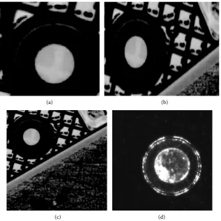
4. Experimental Results

In this section, some experimental results are demonstrated to show the execu-tion-time and accuracy advantages of our improved RCD algorithm, compared with standard RCD algorithm. Four original images are used to evaluate the per-formance of the proposed algorithm. The first three images with the same mark are shown in Figures 4(a)-(c), which have different size 131 124× , 262 153× and 307 307× pixels. The last image Figure 4(d) has another different mark. The radius of the first mark R is 26.5 pixels and the radius of the second mark R is 36.5 pixels. Table 1 describes all parameters used in our experiments. Some

(a) (b)

[image:9.595.216.534.277.595.2]

(c) (d)

Figure 4. Four original images with different size and mark. (a)-(c) Original images with the same mark; (d) Original image with another different mark.

Table 1. All thresholds used in experiments.

f

T Tr Ta Td Tc TrL TrU Tcc

Pure RCD 100,000 0.6 0.25R 1.5 20 R − 5 R + 5 1

Improved

[image:9.595.207.539.656.722.2]

(10)

DOI: 10.4236/am.2019.1010061 857 Applied Mathematics additional variables are defined as following: P denotes the center pixel

(

x y,

)

of detected circle. R is the pre-input radius and r is the radius of detected circle. PN is the number of pixels on the contour of detected circle. C is the circularity of detected circle. Avg T (ms) represents the average running time in millise-cond. Tcc is the threshold of circularity.

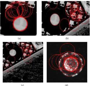
4.1. Locating Mark with Standard RCD Algorithm

In this part the marks will be detected by using standard RCD algorithm. As shown in Figure 5 there are many correct and incorrect circles in images. In Figure 5(c) the true mark circle is not included in the detected possible circles. There is no way to discard the incorrect circles and find the true mark. Accord-ing to the threshold Tc, there are twenty possible detected circles at most, which are drawn in Figure 5. In Tables 2-5 only ten possible circles are described.

(a) (b)

[image:10.595.225.522.275.558.2]

(c) (d)

[image:10.595.206.541.621.734.2]

Figure 5. Locating results using standard RCD algorithm. (a)-(c) The detected results, obtained from Figures 4(a)-(c); (d) The result obtained from Figure 4(d).

Table 2. Ten results shown in Figure 5(a).

P r PN P r PN

(71.039, 81.479) 25.911 404 (70.902, 80.576) 26.225 369

(90.787, 30.734) 28.790 133 (75.500, 83.700) 28.452 138

(70.930, 79.679) 26.190 302 (45.153, 11.418) 27.853 58

(72.391, 81.334) 25.750 383 (71.071, 80.071) 25.014 320.000

(11)

Table 3. Ten results shown in Figure 5(b).

P r PN P r PN

(189.352, 66.432) 26.473 175 (157.550, 47.532) 26.822 170

(194.103, 72.685) 24.486 116 (195.472, 52.751) 24.591 166

(157.036, 36.878) 24.956 151 (223.636, 50.818) 26.623 106

(201.467, 86.570) 23.407 89 (185.626, 41.030) 23.896 143

(169.820, 65.472) 27.184 158 (206.284, 80.524) 27.742 67

(71.982, 81.718) 25.382 379 (62.561, 16.912) 23.763 66

Table 4. Ten results shown in Figure 5(c).

P r PN P r PN

(34.786, 163.67) 27.257 150 (252.645, 48.271) 28.241 122

(177.100, 43.500) 28.500 148 (103.150, 122.58) 23.413 74

(69.098, 179.443) 25.349 103 (205.563, 55.500) 26.300 137

(145.883, 32.260) 27.740 151 (167.003, 42.453) 26.043 204

(216.647, 44.956) 25.610 97 (148.500, 13.571) 27.472 119

(71.982, 81.718) 25.382 379 (62.561, 16.912) 23.763 66

Table 5. Ten results shown in Figure 5(d).

P r PN P r PN

(116.345, 107.928) 33.594 286 (115.135, 107.68) 34.296 318 (116.459, 106.745) 34.481 348 (137.832, 112.68) 33.834 102 (116.271, 107.794) 34.310 337 (116.256, 106.40) 33.951 309

(132.030, 109.909) 35.091 83 (107.256, 129.41) 34.519 101

(116.398, 101.856) 35.538 108 (116.355, 106.31) 34.913 325

4.2. Locating Mark with Improved RCD Algorithm

(12)

(a) (b) (c) (d)

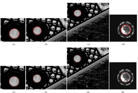
[image:12.595.57.542.61.389.2]

(e) (f) (g) (h)

[image:12.595.208.539.452.502.2]

Figure 6. Results obtained by using our improved RCD algorithm and circularity. (a)-(d) Results obtained without calculating minimal circularity; (e)-(h) Results obtained by calculating the minimal circularity.

Table 6. Results shown in Figure 6(a).

P r PB c

(72.313, 81.737) 26.795 309 0.8077

[image:12.595.209.539.538.636.2]

(71.500, 80.500) 26.163 392 0.1288 Selected As true

Table 7. Results shown in Figure 6(b).

P r PN c

(71.404, 82.005) 26.291 356 0.8077

(71.369, 81.622) 27.132 253 0.1288 Selected As true

(71.194, 81.403) 27.016 272 0.2732

(71.570, 80.779) 26.903 290 0.1548

Table 8. Results shown in Figure 6(c).

P r PN c

(74.985, 81.435) 27.104 257 0.6047

(13)

[image:13.595.206.540.89.175.2]

Table 9. Results shown in Figure 6(d).

P r PN c

(114.992, 108.471) 34.629 356 0.0595 Selected As true

(14.192, 107.192) 34.529 376 0.0985

(116.826, 106.174) 34.699 461 0.2000

(116.500, 108.500) 34.821 383 0.1547

Table 10. Time performance comparison between standard RCD and the improved RCD

in terms of milliseconds.

Original Images Avg T (RCD) Avg T (improved RCD)

Figure 4(a) 77.8 ms 121 ms

Figure 4(b) 466.8 ms 478.2 ms

Figure 4(c) 1172.8 ms 710 ms

Figure 4(d) 148.2 ms 145 ms

radius 26.951 pixels is detected. In Table 9 the true circle with center pixel (114.992, 108.471) and radius 34.629 pixels is detected.

4.3. Comparing the Execution-Time

In order to compare the execution-time, all concerned experiments are per-formed on the Intel i5-5200U CPU with 2.20 GHz and 8 GB RAM. The adopted operating system is MS-Windows 7 and the programming environ-ment is VS2010. In order to accurately evaluate the execution-time, we run each image 100 times and calculate the average time in Table 10. For locat-ing mark in small images, the execution-time is almost the same for both al-gorithms. The time will be significantly reduced, when the mark is detected in a larger and complex image.

5. Conclusions

This paper has presented the proposed improved RCD strategy to improve the performance of execution-time and the accuracy of detection. The refined me-thod can suppress the interference between different objects significantly. After calculating minimal circularity, the true mark will be located efficiently and ac-curately. The experimental results demonstrate that the proposed improved RCD improves significantly the accuracy of detection. Experimental results also demonstrate that the proposed algorithm provides a considerable execution-time improvement. The algorithm has significant execution-time superiority in large and complex image.

[image:13.595.207.538.218.303.2]

(14)

Founding

This article is supported by Science and Technology Project of Fujian Provincial Department of Education under contract JAT170917 and Youth Science and Research Foundation of Chengyi College Jimei University under contract C16005.

Conflicts of Interest

The authors declare no conflicts of interest regarding the publication of this pa-per.

References

[1] Gonzalez, R.C. and Woods, R.E. (1992) Digital Image Processing. Addison Wesley, New York.

[2] Forsyth, D.A. (2002) Computer Vision: A Modern Approach. Prentice-Hall, New Jersey.

[3] Leavers, V.F. (1993) Survey: Which Hough Transform. CVGIP: Image Under-standing, 58, 250-264. https://doi.org/10.1006/ciun.1993.1041

[4] Duda, R.O. and Hart, P.E. (1972) Use of the Hough Transformation to Detect Lines and Curves in Pictures. Communications of the ACM, 15, 11-15.

https://doi.org/10.1145/361237.361242

[5] Xu, L. and Oja, E. (1993) Randomized Hough Transform (RHT): Basic Mechan-isms, Algorithms, and Computational Complexities. CVGIP: Image Understanding, 57, 131-154. https://doi.org/10.1006/ciun.1993.1009

[6] Chen, T.C. and Chung, K.L. (2001) An Efficient Randomized Algorithm for De-tecting Circles. Computer Vision and Image Understanding, 83, 172-191.

https://doi.org/10.1006/cviu.2001.0923

[7] Fischer, M.A. and Bolles, R.C. (1981) Random Sample Consensus: A Paradigm to Model Fitting with Applications to Image Analysis and Automated Cartography.

Communications of the ACM, 24, 381-395. https://doi.org/10.1145/358669.358692

[8] Jia, L.Q., Peng, C.Z., Liu, H.M. and Wang, Z.H. (2011) A Fast Randomized Circle Detection Algorithm. International Congress on Image and Signal Processing, 4, 835-838. https://doi.org/10.1109/CISP.2011.6100372

[9] Gomes, J. and Velho, L. (1997) Image Processing for Computer Graphics. Sprin-ger-Verlag, New York. https://doi.org/10.1007/978-1-4757-2745-6

[10] Gonzalez, R.C. and Woods, R.E. (2008) Digital Image Processing. Pearson Prentice Hall, New Jersey.

[11] Davies, E.R. (2005) Machine Vision: Theory Algorithms Practicalities. Morgan Kaufmann, San Francisco.