Error control for hp adaptive approximations of semi definite eigenvalue problems

ERROR CONTROL FOR hp-ADAPTIVE APPROXIMATIONS OF SEMI-DEFINITE EIGENVALUE PROBLEMS

STEFANO GIANI, LUKA GRUBIˇSI ´C, AND JEFFREY S. OVALL

Abstract. We present reliable a-posteriori error estimates forhp-adaptive finite element approx-imations of semi-definite eigenvalue/eigenvector problems. Our model problems are motivated by the applications in photonic crystal eigenvalue computations. We present detailed numerical ex-periments confirming our theory and give several benchmark results which could serve the purpose of numerical testing of other adaptive procedures.

1. Introduction

Accurate computation of eigenvalues of elliptic differential operators remains a highly challenging numerical task regardless of the considerable research effort which has been recently invested in it. For operators for which particular solutions of (local) eigenvalue problems are known explicitly, a

modified method of particular solutions such as that described [11] seems to be the most efficient

means to deliver as many accurate digits in computed eigenvalues as possible. However, the class of operators to which this method can be successfully applied is limited, and does not include many operators having discontinuous or anisotropic coefficients on the highest-order derivatives (cf. [15]).

For this broader class of problems, hp-adaptive discontinuous Galerkin (DG) methods currently

appear to be the most efficient, as measured by flops per accurate digit delivered, to compute the eigenvalues/eigenvectors, see [18] and the references therein. In the present work, we put forth an

hp-adaptive continuous Galerkin method which aims at similar practical efficiency, while supplying a much more robust error estimation theory for eigenvalue and invariant subspace computations.

The difficulty which is associated with eigenvalue/eigenvector problems for differential operators with discontinuous coefficients partly stems from the nonlinear nature of the eigenvalue problem itself and partly from the inherent singularities which the eigenvectors can posses. For instance it is known that eigenvectors of such operators can exhibit arbitrarily bad singularities, e.g. being in the Sobolev space H1+β for arbitrarily small β >0, see [12, 13, 23] and references therein.

In this paper we are interested in the elliptic eigenvalue problems which arise in connection with the inverse problems of nondestructive sensing and in the modeling of two phased optic materials (e.g. photonic crystals), see [3–5]. The main feature of these problems is that they are defined by differential operators which have jumping coefficients. Further, these problems depend on a parameter describing material properties. Sometimes varying of the parameter can change dramatically the spectral properties of the eigenvalue problem, e.g. introduce zero eigenvalues.

Computing a zero eigenvalue with floating point arithmetic is always a challenge. The difficulty arises because the important geometric properties, like orthogonality, are only “approximately” realized. Subsequently, numeric pollution might appear. Also, simply shifting away from zero will not solve the problem since shifting strategies do not guarantee high relative numerical accuracy of the computed results.

Date: April 14, 2012.

2000Mathematics Subject Classification. Primary: 65N30, Secondary: 65N25, 65N15.

We tackle this problem using the techniques of relative perturbation theory, for eigenvalues and pseudo inverses, from matrix analysis. In particular we define the penalization based positive defi-nite approximation of the initially given semi defidefi-nite differential operator (because of Neumann or periodic boundary condition). We study the spectral convergence of the penalization approxima-tion in the limit of the large penalty parameter using the analytic technique from [20]. Assuming a basis for the null space of the operator is explicitly known, we show how to set the penalty parame-ter which ensures the numerical orthogonality of the computed approximations onto the null space of the operator. This is particularly important for eigenvalue problems (e.g. in photonic crystal applications) where the null space intersects the finite element space only trivially.

The estimation theory from [21] is based on the technique to reduce the study of the approxima-tion properties of a Galerkin eigenvalue approximaapproxima-tion to the study of the Galerkin approximaapproxima-tion of the solution of the associated source problem, e.g. to the study of the inverse of the associated positive definite differential operator. We generalize this approach, using the theory from [19], to allow us to treat semi-definite eigenvalue problems by reducing them to the study of the generalized inverse of the associated singular operator.

We treat the inverse/pseudo inverse of our operator using the estimation theory for the continuous

hp-adaptive approximations to the solution of a source problem from [25]. We show efficiency and

reliability estimates. In particular, we point out that our reliability constant is independent of the

polynomial degree and depends only on the regularity parameter of thehp-adaptive approximation.

Finally we report on an extensive numerical study of the proposed estimator. In particular we show that our estimator is robust with respect to the dependence on the parameter of the problem even in the case when for some singular values of the parameter the problem changes type (positive definite problem becomes semi-definite). Also, we show that our estimator is robust with respect to the size of the jump in the coefficients of the differential operator.

We assess the robustness of the estimator by computing the effectivity quotients of the error with the estimator. To approximate the error we either use explicit solutions, when available, or highly accurate numerical solutions. Such highly accurate solutions have been computed by a discontinuous Galerkin method. The accuracy of these benchmark solutions have been assessed by an expensive goal oriented estimator as described in [18].

The paper is organized as follows: In Section 2 we describe the two classes of model prob-lems under consideration, outline the basic theory of such probprob-lems, discuss the hp-discretization,

and introduce the key concept of approximation defects and it relation to discretization errors in

eigenvalue and invariant subspace computations. Section 3 contains the key results concerning a practical estimation of eigenvalue and invariant subspace discretization errors. Extensive and de-tailed experiments which demonstrate the performance of our approach are provided in Section 4. Finally, in Section 5 we briefly summarize the key points of this work, and indicate the directions in which we expect further progress to be made.

2. Model problem and approximation defects

We are interested in the eigenvalue problems of the form:

Find (λ, ψ)∈R× Hso that B(ψ, v) =λ(ψ, v) andψ6= 0 for all v∈ H ,

(2.1)

whereH is a real or complex Hilbert space containing the L2_{-integrable functions, B is a positive} semi-definite bilinear or sesquilinear form, and (v, w) is the L2 inner-product on H. We use the

standard notation v ⊥w to denote that (v, w) = 0, v ⊥W to denote that v ⊥w for all w ∈ W,

and V ⊥W to denote thatv⊥W for allv ∈V. We consider two classes of problems:

Definition 2.1 (Type I Problems). Let Ω ⊂ R2 be a bounded polygonal region, possibly with re-entrant corners. We takeH:=H1(Ω) as the usual first order Sobolev space over R, and define

(2.2) B(w, v) =

Z

Ω

A∇w· ∇vdx,

where A ∈ [L∞(Ω)]2×2 is uniformly positive definite a.e. As a practical matter, we will further

assume thatA is piecewise-constant on some polygonal partition of Ω.

Definition 2.2 (Type II Problems). Let Γ =Z2 be a periodicity lattice and letT2 =R2/Γ denote

the torus in two dimensions. We define H = H1(T2) as the usual first order (periodic) Sobolev

space over C. For fixedκ∈R2, we define eigenvalue problem defined by the forms

(2.3) B(u, v) =

Z

T2

A(∇+ iκ)u·(∇+ iκ)vdx.

If we want to emphasize that B corresponds to a Type II problem, we will use κ as a subscript,

e.g. Bκ. The matrixA∈[L∞(T2)]2×2 is assumed to be Hermitian positive definite a.e., and again,

as a practical matter it is assumed to be piecewise constant on some polygonal partition of T2.

Here and elsewhere, we use the following standard notation for norms and seminorms: fork∈N

and a domain S we denote the standard norms and semi-norms on the Hilbert spaces Hk(S) by

kvk2_k,S = X |α|≤k

kDαvk2_S |v|2_k,S = X |α|=k

kDαvk2_S ,

(2.4)

wherek · kS denotes theL2 norm onS. WhenS = Ω orS=T2 we omit it from the subscript. We

also use the notation

|||u|||=B(u, u)1/2 , |||u|||κ =Bκ(u, u)1/2, κ∈R2,

to denote the energy semi-norms ofu∈ H.

2.1. Properties of semidefinite model eigenvalue problems. We define Ker(B) := {u ∈ H: B(u, u) = 0} and letN :H →Ker(B) be theL2-orthogonal projection. Noting that Ker(B) is a closed subspace, we also defineQ=I−N :H →Ker(B)⊥ as theL2-orthogonal projection onto

theL2-orthogonal complement of Ker(B). BothQ and N are spectral projections for the positive

semi-definite self-adjoint operator Awhich is defined in the sense of Kato by

(A1/2u,A1/2v) =B(u, v) u, v∈ H

and Dom(A1/2) =H.

For Type I problems, it is clear that Ker(B) operator consists of the constant functions—these are the eigenfunctions associated with the simple eigenvalue 0. As any reasonable discrete space

V will contain the constant functions, this class of problems exemplifies the more general case in

which Ker(B) ⊂ V. For Type II problems it is clear that, for κ ∈ 2πZ2, Ker(B) is spanned by

ψ0 =e−iκ·x—this is the unique solution of (∇+iκ)ψ= 0. As before, these are the eigenfunctions

associated with the simple eigenvalue 0. The restriction on κ is solely to satisfy the periodicity

conditions. When κ=0, we are back to the case of constant functions in the kernel, so Ker(B)⊂

V. In the more interesting case, κ ∈ 2πZ2 _{\ {0}, for the finite element spaces V described in}

Subsection 2.2, it is apparent that Ker(B)∩V = {0}. For either type of model problem the

dimension of the kernel is (at most) one, but we also consider the more general situation when

Let σ > 0 be given, and define Bσ(u, v) =B(u, v) +σ(u, N v). For a functionf ∈ L2 we may consider two related source problems:

Find u+(f)∈ H such thatB(u+(f), v) = (Qf, v) for everyv∈ H ,

Find uσ(f)∈ H such thatBσ(uσ(f), v) = (f, v) for everyv∈ H .

The choice of notation u+_{(f) is due to the fact that, from the algebraic point of view, we are}

computing the action of the generalized inverse of the operator which is defined by the formB on

the vectorf ∈L2. The latter of these offers an alternative for computing the inverse, via Tikhonov regularization, with “penalty parameter” σ. It holds that

lim

σ→∞u

σ_{(f) =u}+_{(f) ,}

and we have the estimate

0≤ |||uσ(f)−u+(f)|||2_σ = f, uσ(f)− f, u+(f)≤ C

σ f, f

,

for the speed of convergence—see [20, Theorem 4.3] and note thatN is a spectral projection. The

constantC is independent of f, and we use|||v|||2_σ =Bσ(v, v).

For this paper we assume that the operator A is such that 0 is an isolated eigenvalue. This

means that we can number the nonzero eigenvalues of the operator Aby

(2.5) 0< λ1 ≤λ2 ≤ · · · ≤λq≤ · · · .

Here we count the nonzero eigenvalues according to their multiplicities. Solutions of the variational eigenvalue problems (2.1) are attained by the positive sequence of eigenvalues (2.5) and a sequence of eigenvectors (ψi)i∈N such that

B(ψi, v) =λi(ψi, v), ∀v∈ H, and (ψi, ψj) =δij .

(2.6)

Here and below we count the eigenvalues according to their multiplicity. Furthermore, the sequence (λi)i∈N has no finite accumulation point and

L2(Ω) = Ker(B)⊕Cls(span{ψj : j ∈N}) .

2.1.1. Relationship between eigenvalues/vectors of B and Bσ. In this section we summarize the

results of [20] which are relevant for this paper. First note that the form Bσ is positive definite, therefore we use

0< λ1(σ)≤λ2(σ)≤ · · · ≤λq(σ)≤ · · ·

to denote the eigenvalues of the eigenvalue problem for Bσ, and (ψi(σ))i∈N denotes a sequence of

eigenvectors which is numbered as in (2.5) and (2.6). Standard monotonicity results (e.g. [27]) imply that

λj(σ)≤λj, j∈N

and λj(σ) → λj as σ → ∞, together with multiplicity. Furthermore, a similar result holds for

spectral projections.

LetE(λq) be theL2orthogonal projection onto the space span{ψj : j= 1,· · ·, q}and letEσ(λq)

be its orthogonal projection onto span{ψi(σ) : λi(σ)≤λq}. We have the following technical result,

which follows from [20, Theorem 3.3], [20, Corollary 3.8] and [20, Theorem 4.3]:

Lemma 2.3. Let m ∈ N be given such that λm < λm+1. Then there exists a parameter σ0 and

constants c1,m,C1,m andC2,m such that the following estimates hold

c1,m

σ ≤

m

X

i=1

λj−λj(σ)

λj ≤

C1,m σ

(2.7)

kE(λ_m)−Eσ(λm)kHS ≤

C_√2,m σ .

(2.8)

for allσ > σ0. The constantsC1,mandC2,mdepend solely on the distance betweenλm andλm+1 and

the regularity properties of Ker(B) where as the constant c1,m depends on the regularity properties

of Ker(B) and the quotient λ1/λm. The norm k · kHS is the Hilbert-Schmidt norm on the space

of compact operators (Hilbert-Schmidt operators are those compact operators A such that operator

A∗A has a finite trace and thenkAkHS =

p

tr(A∗A)).

2.2. Discrete eigenvalue/eigenvector approximations. We discretize (2.1) usinghp-finite el-ement spaces, which we now briefly describe. LetT =Th be a triangulation of Ω with the

piecewise-constant mesh function h :Th → (0,1), h(K) = diam(K) for K ∈ Th. Throughout we implicitly

assume that the mesh is aligned with all discontinuities of the data A. Given a piecewise-constant distribution of polynomial degrees,p:Th →N, we define the space

V =V_hp ={v∈ H ∩C(Ω) : v_K∈Pp(K) for each K∈ Th},

wherePjis the collection of polynomials of total degree no greater thanjon a given set. Suppressing

the mesh parameterhfor convenience, we also define the set of edgesEinT, and distinguish interior edgesEI, and edges on the boundaryEN. Additionally, we letT(e) denote the one or two triangles

having e ∈ E as an edge, and we extend p to E by p(e) = max_K∈T(e)p(K). As is standard, we assume that the family of spaces satisfy the following regularity properties on Th and p: There is

a constant γ >0 for which

(C1) γ−1[h(K)]2 ≤area(K) forK ∈ T,

(C2) γ−1(p(K) + 1)≤p(K0) + 1≤γ(p(K) + 1) for adjacent K, K0∈ T,K∩K0 6=∅.

It is really just a matter of notational convenience that a single constant γ is used for all of these upper and lower bounds. The shape regularity assumption (C1) implies that the diameters of adjacent elements are comparable.

In what follows we consider the discrete versions of (2.1):

Find (ˆλ,ψˆ)∈R×V such that B( ˆψ, v) = ˆλ( ˆψ, v) for all v∈V .

(2.9)

We also assume, without further comment, that the solutions are ordered and indexed as in (2.5), with ( ˆψi,ψˆj) =δij. That is to say we have

0<λˆ1≤ˆλ2 ≤ · · · ≤λˆNZ.

More to the point, we assume that either Ker(B)∩ V = {0} or Ker(B) ⊂ V and obviously

NZ ≤dimV.

We are interested in assessing approximation errors in collections of computed eigenvalues and associated invariant subspaces. Let sm = {µk}m_k=1 ⊂ (a, b) be the set of all eigenvalues of B,

counting multiplicities, in the interval (a, b), a > 0, and let Sm = span{φk}mk=1 be the associated invariant subspace, with (φi, φj) =δij. The discrete problem (2.9) is used to compute corresponding

approximations ˆsm ={µˆk}km=1 and ˆSm = span{φˆk}mk=1, with ( ˆφi,φˆj) =δij.

Remark 2.4. Whensm consists of the smallestmpositive eigenvalues, we use the absolute labeling

sm = {λk}m_k=1 and Sm = span{ψk}m_k=1 instead of the relative labeling involving (µk, φk); and the

2.3. Approximation defects. Let the finite element space V ⊂ H be given and let ˆsm and ˆSm

be the approximations which are computed fromV. We define theapproximation defects in ˆsm,Sˆm

as:

η2_i( ˆSm) = max

S⊂_Smˆ dimS=m−i+1

min

f∈S f6=0

|||u+(f)−uˆ+(f)|||2 |||u+_(f)|||2 , (2.10)

whereu+(f) and ˆu(f) satisfy:

B(u+(f), v) = (Qf, v) for everyv∈ H

(2.11)

B(ˆu+(f), v) = (Qf, v) for everyv∈V .

(2.12)

We will argue below that such approximation defects are very useful for estimating the error in ˆsm

as an approximation of sm (and ˆSm as an approximation of Sm).

Of course,u+(f), and henceηi, cannot be computed, so we must efficiently and reliably estimate

these quantities. For positive definite forms, we have shown in [21] how to use hierarchical basis error estimators (cf. [9]) to efficiently and reliably estimateηi in the case of low-orderh-elements;

and in [17] how to similarly use residual-based error estimators (cf. [14]) in the case ofhp-elements. The present work extends the latter approach to the case of semi-definite forms, and we elaborate on the details in Section 3.

We will state the following geometrical lemma, which follows from [19], and indicates what type of information is encoded in the approximation defects.

Lemma 2.5. Let Cm ={ψ∈Ker(B) : ψ⊥Sˆm} and let ηm( ˆSm)<1. Then

Ker(B) = (Ker(B)∩Sˆm)⊕ Cm.

The approximation defects are related to the eigenvalue error in the following way. Assume that ˆS_m is the span of first m ∈N eigenvectors of (2.5) then we have the following efficiency and

reliability result.

Theorem 2.6. Let B(·,·) be the any of the semi-definite forms given in (2.2) and (2.3) and let

λ_m< λ_m+1. If Sˆm= span{ψˆ1,· · ·,ψˆM} is such that

ηm( ˆSm) 1−ηm( ˆSm)

< λm+1−λˆm

λ_m+1+ˆλm

then

(2.13)

ˆ

λ1

2ˆλm m

X

i=1

η_i2( ˆSm)≤ m

X

i=1 ˆ

λi−λi

ˆ

λi

≤C_M m

X

i=1

η2_i( ˆSm).

The constantCM,depends solely on the relative distance to the unwanted component of the spectrum (e.g. λM−λM+1

λ_M+λ_M+1).

Proof. The fact that 0<λˆi,i= 1,· · ·m and Lemma 2.5 imply the conclusion ˆSm ⊥Ker(B). The problem can now be reduced to the study of the positive definite form

B∞(u, v) =B(u, v), u, v∈Dom(B∞) ={ψ∈ H : ψ⊥Ker(B)}.

Furthermore, we have that

η2_i( ˆSm) =ηi,2∞( ˆSm)

where η_i,2_∞( ˆSm) denotes the approximation defects for the form B∞ and the subspace ˆSm ⊂

Dom(B∞) as defined in [21]. The statement of the theorem follows by [8, Theorem 3.10]. Q.E.D.

The constant CM is given by an explicit formula which is a reasonable practical overestimate,

see [8, 21] for details. A similar results holds for the eigenvectors. We point the interested reader to [21, Theorem 4.1 and equation (3.10)] and [8, Theorem 3.10].

Remark 2.7. Ifλ1=λm, then the constant ˆλ1/2ˆλm in (2.13) can be replaced by 1.

3. Practical error estimators for the hp-adaptive method

3.1. The Case Ker(B) ⊂ V. This case covers all Type I problems, as well as Type II problems

whenκ=0. When Ker(B)⊂V, we work directly with the approximation defects from (2.10). We

have the following modification of [17, Lemma 3.4].

Lemma 3.1. It holds that

1 1 +Dl

m

X

i=1 ˆ

µ−_i 1|||u+(ˆµiφˆi)−uˆ+(ˆµiφˆi)|||2≤ m

X

i=1

η_i2( ˆSm)≤ m

X

i=1 ˆ

µ−_i1|||u+(ˆµiφˆi)−uˆ+(ˆµiφˆi)|||2 .

(3.1)

The constant Dl was defined in [17].

We must estimate|||u+(ˆµiφˆi)−uˆ+(ˆµiφˆi)|||2 for each Ritz vector, where ˆSm = span{φˆ1, . . . ,φˆm}is

our approximation ofSm = span{φ1, . . . , φm}. We modify key results from [17], which were stated

only for in the positive definite case to our context. The identity ˆu+(ˆµiφˆi) = ˆφi, makes our job

easier. We define the element residuals Ri forK ∈ T, and the edge (jump) residualsri for e∈ E,

by

Ri|K= ˆµiφˆi+∇ ·A∇φˆi , ri|e=

(

−(A∇φˆi)_|K ·nK−(A∇φˆi)|K0 ·nK0 , e∈ EI

−(A∇φˆi)_|K ·nK , e∈ EN

,

(3.2)

for Type I problems and Type II problems withκ=0. For interior edgese∈ EI,K andK0 are the

two adjacent elements, having outward unit normals nK and nK0, respectively; and for boundary

edges e∈ EN,K is the single adjacent element, having outward unit normalnK. We note thatR

is a polynomial of degree no greater than p(K) on K, and r is a polynomial of degree no greater thanp(e)−1 one.

Our estimate ofε2

i =

P

K∈T ε2i(K)≈ |||u+(ˆµiφˆi)−uˆ+(ˆµiφˆi)|||2 is computed from local quantities,

ε2_i(K) =

h(K)

p(K)

2

kRik20,K +

1 2

X

e∈EI(K)

h(e)

p(e)krik 2 0,e+

X

e∈EN(K)

h(e)

p(e)krik 2 0,e ,

(3.3)

whereEI(K) andEN(K) denote the interior edges and boundary edges of K, respectively.

The following analogues of [17, Lemma 4.1, Lemma 4.2] carry over directly in this case.

Lemma 3.2. The following holds for Type I and Type II problems for which Ker(B) ⊂V. There is a constant C > 0, depending only on the hp-constant γ and λmin(A), such that |||u+(ˆµiφˆi)−

ˆ

u+(ˆµiφˆi)|||2 ≤ Cεi2. Furthermore, for any > 0, there is a constant c =c() > 0, depending only on the hp-constant γ andkBk, such that ε2

i(K)≤cpK2+2|||u+(ˆµiφˆi)−uˆ+(ˆµiφˆi)|||2ωK.

With this we have

Theorem 3.3. Under the assumptions of Theorem 2.6, we have the following upper- and lower-bounds on eigenvalue error,

(3.4) C1

m

X

i=1 ˆ

λ−_i 1ε2_i ≤ m

X

i=1 ˆ

λi−λi

ˆ

λi

≤C2 m

X

i=1 ˆ

λ−_i 1ε2_i .

The constant C1 depends solely on the ratio λˆ1/(2ˆλ2), the hp-regularity constant γ, the continuity

constant kBk, and the maximal polynomial degree p¯ = maxK∈T p(K). The constant C2 depends

solely on the relative distance to the unwanted component of the spectrum, thehp-regularity constant

3.2. The Case Ker(B) ∩ V = {0}. Although the Type II problems of this sort have a

one-dimensional kernel, we consider the more general situation of ak-dimensional kernel. Here we

em-ploy the penalized formBσ_{, which yields a positive definite eigenvalue problem. Theσ-dependence}

of the corresponding discrete eigenpairs (ˆλi,ψˆi) = (ˆλi(σ),ψˆi(σ)) or (ˆµi,φˆi) = (ˆµi(σ),φˆi(σ))

should be understood even when it is suppressed for notational convenience. Also, we use the notation ˆE(λm) to denote the orthogonal projection onto the space span{ψˆi(σ) : ˆλi(σ)≤λm}

We let {z1, . . . , zk} be an orthonormal basis of eigenfunctions for Ker(B), so

Bσ(u, v) =B(u, v) +σ(u, N v) =B(u, v) +σ

k

X

j=1

(u, zj) (zj, v)

(3.5)

If{v1, . . . , vN}is a standard (locally supported) basis forV, it is clear from (3.5) that the stiffness

associated with Bσ and this basis will be the sum of a sparse matrix and one which is of (at most) rankk. In this sense the stiffness matrix is “data-sparse”, because its action on a vector is anO(N) computation.

Using a Cauchy inequality (with δ), we see that

|||v|||2_σ ≥(1−δ)λmin(A)|v|2_1,T2 −

1

δ −1

λmax(A)kκk2`2kvk

2

0,T2 +σkN vk2_0,T2 ,

for any δ >0. So although Bσ is not coercive with respect to| · |1,T, in the sense that we cannot

guarantee that |||v|||σ ≥m0|v|1,T for somem0 which is independent ofv∈ H, a G˚arding does hold,

|||v|||2_σ+ρkvk2_0,T2 ≥m20|v|2_1,T2 ,

withρ= (1/δ−1)λmax(A)kκk2`2 and m

2

0 = (1−δ)λmin(A), for example. In our derivation of error estimates for Type II withκ6=0, we consider the (further) modified form

Bσ,ρ(u, v) =Bσ(u, v) +ρ(u, v) ,

with corresponding norm |||v|||σ,ρ ≥ m0|v|1,T. It is clear that (λ, ψ) = (λ(σ), ψ(σ)) is an eigenpair

forBσ if and only if (λ+ρ, ψ) is an eigenpair for Bσ,ρ, and that the analogous assertion holds on the discrete level as well. This spectrum-shifting trick has been used elsewhere (cf. [16]) for similar theoretical arguments, and we will see below that it has no effect on practical implementation.

We motivate our choice of error estimates as follows: Suppose that (ˆλ,ψˆ) ∈ R+×V satisfies

Bσ( ˆψ, v) = ˆλ( ˆψ, v) for allv ∈V. As stated above,Bσ,ρ( ˆψ, v) = (ˆλ+ρ) ( ˆψ, v) for all v∈V. We set

f = (ˆλ+ρ) ˆψ and defineu(f)∈ Hand ˆu(f)∈V by

Bσ,ρ(u(f), v) = (f, v) for all v∈ H , Bσ,ρ(ˆu(f), v) = (f, v) for allv∈V .

It is clear that ˆu(f) = ˆψ. We now go through the usual steps for deriving residual-based error

estimates for boundary value problems. For any v∈ H and ˆv∈V,

Bσ,ρ(u(f)−uˆ(f), v) =Bσ,ρ(u(f)−uˆ(f), v−vˆ) = (f, v−ˆv)−Bσ,ρ(ˆu(f), v−ˆv)

=

 _λˆ_ψˆ_−σ

k

X

j=1

( ˆψ, zj)zj , v−vˆ



₋B( ˆψ, v−ˆv)

B( ˆψ, v−vˆ) = X

K∈T

Z

∂K

A(∇+iκ) ˆψ·n(v−vˆ)ds−

Z

K

(∇+iκ)·A(∇+iκ) ˆψ(v−ˆv)dx

We emphasize that the quantity on the right-hand side is independent ofρ. Choosing the element and edge residuals

Rσ|K =



_λˆ_ψˆ_{+ (∇+iκ)·A(∇+iκ) ˆψ−σ}

k

X

j=1

( ˆψ, zj)zj

 

|K

(3.6)

rσ|e=

(

−(A(∇+iκ) ˆψ)_|K ·nK−(A(∇+iκ) ˆψ)_|K0 ·nK0 , e∈ EI

−(A(∇+iκ) ˆψ)_|K ·nK , e∈ EN

,

(3.7)

we naturally define the error estimate ε2_σ ≈ |||u(f)−uˆ(f)|||2_σ,ρ by

ε2_σ = X

K∈T

ε2_σ(K) (3.8)

ε2_σ(K) =

h(K)

p(K)

2

kRσk2_0,K+1 2

X

e∈EI(K)

h(e)

p(e)kr

σ_k2 0,e+

X

e∈EN(K)

h(e)

p(e)kr

σ_k2 0,e .

(3.9)

At this stage, Cauchy-Schwarz inequalities (both continuous and discrete) and interpolation error estimates yield

|||u(f)−uˆ(f)|||2_σ,ρ≤Cεσ|u(f)−uˆ(f)|1,T≤

C m0

εσ|||u(f)−uˆ(f)|||σ,ρ ,

for some C which depends only on the mesh parameter γ. From this we deduce, via the obvious

bound|||u(f)−uˆ(f)|||σ ≤ |||u(f)−uˆ(f)|||σ,ρ, that

Lemma 3.4. If (ˆλ,ψˆ)∈R+×V is a discrete eigenpair forBσ, and we choose f = (ˆλ+ρ) ˆψ for ρ

sufficiently large (see above discussion), then

|||u(f)−uˆ(f)|||σ ≤

C m0

εσ ,

where C depends only on the mesh parameter γ, and m0 depends only on λmin(A).

The (strong) residuals Rσ and rσ are naturally functions on R+×V, with Rσ =Rσ(ˆλ,ψˆ) and

rσ =rσ(ˆλ,ψˆ) given in (3.6)-(3.7). For a collection of discrete eigenpairssm ={(ˆµi,φˆi) : 1≤i≤m}

forBσ we define the corresponding residuals Rσ,i=Rσ(ˆµi,φˆi) andrσ,i=rσ(ˆµi,φˆi), and defineεi,σ

from Rσ,i and rσ,i as in (3.8)-(3.9). We remark that, although we have stated these definitions in

the relative numbering (a collection anywhere in the spectrum), Theorem 3.5 concerns the first m

positive eigenvalues, and therefore uses the absolute numbering (ˆλi,ψˆi). We now state the main

theorem in this context as a combination of Lemma 2.3 and [17, Theorem 4.4].

Theorem 3.5. Let Ker(B)∩V ={0} and let m∈N be such thatλm< λm+1. Then forσ > σ0 m

X

i=1

|ˆ_{λi(σ)−λi|}

λi ≤

C2 m

X

i=1 ˆ

λ−_i 1(σ)ε2_i,σ+C1,m

σ

(3.10)

kE(λ_m)−Eˆσ(λm)kHS ≤C3

v u u

tXm

i=1 ˆ

λ−1_i (σ)ε2

i,σ+

C_√2,m σ .

(3.11)

The constants C1,m and C2,m are precisely as in Lemma 2.3, and the constants C2 and C3 depend

Proof. The proof of (3.10) is an obvious combination, by the use of the triangle inequality, of

Lemma 2.3, Lemma 3.4 and [17, Theorem 4.4]. We will concentrate on proving (3.11). Let σ0 be

as given by Lemma 2.3. Recall that the formBσ_{(·,·) is positive definite. Then using [20, Theorem}

3.3] we establish that there exists a constant CS which depends solely on the distance between

λm+1(σ) and ˆλm(σ) such that

kEσ(λm)−Eˆσ(λm)kHS ≤CS

v u u

tXm

i=1 η2_i(σ).

Here η2_i(σ) is defined by the formula

η_i2(σ) = max S⊂_Sˆ

m dimS=m−i+1

min

f∈S f6=0

|||u(f)−uˆ(f)|||2_σ |||u(f)|||2

σ

, i= 1,· · · ,m,

and ˆS_m = span{ψˆi(σ) : ˆλi(σ)≤λm}. Assume that the spaceV_hp is such that the assumptions of

Theorem 2.6 hold for the form Bσ, that is let

η_m(σ) 1−η_m(σ) <

λ_m+1(σ)−λˆm(σ)

λm+1(σ) + ˆλm(σ)

then dim ˆSm =m. The conclusion of the theorem now follows from the triangle inequality for the Hilbert-Schmidt norm and Lemmas 2.3 and 3.4. Q.E.D.

Theorem 3.5 implies that it would be reasonable to setσ= (dimVu)−2as our penalty parameter, whereu≈10−16 is the unit roundoff. Recall that the scalar product in the finite element spaceV

can be computed up to the accuracy of O(dimVu) and thatkE(λ_m)−Eσ(λm)kHS is a measure of the sine of the largest angle which a vector from Ran(E(λ_m)) = span{ψi : λi ≤λm}can have with

a vector from Ran(Eσ(λm)) = span{ψi(σ) : λi(σ)≤λm}. Settingσ= (dimVu)−2implies that the

angle between eigenvectorsψi(σ),i= 1,· · ·,mof the auxiliary problem and the target eigenvectors

ψi, i = 1,· · ·,m is on the order of the accuracy with which a sine of an angle can be evaluated.

Subsequently, for an arithmetic with such a rounding constantu vectors ˆψi(σ),i= 1,· · · ,mare as

good approximations ofψi,i= 1,· · ·,mas they are of ψi(σ), i= 1,· · ·,m.

4. Experiments

In this section we have collected numerical results regarding our a posteriori error estimator with the clear aim to show the efficiency of the error estimator and the exponential converge of the error

on a sequence of hp-adapted meshes. Following [7], we assume an error model of the form

ˆ

λi =λi+Ce−2α

√ DOFs

for problems whose eigenfunctions are expected to be smooth, and

ˆ

λi =λi+Ce−2α

3

√ DOFs_,

for problems such as those on non-convex polygonal domains and/or discontinuous coefficients,

whose eigenfunctions are expected to have isolated singularities. The constants C and α are

de-termined by least-squares fitting, and α is reported for each problem. Plots are given of the total relative error, its a posteriori estimate, and the associated effectivity index, shown, respectively, below:

m

X

i=1 ˆ

λi−λi

ˆ λi , m X i=1 ˆ

λ−_i 1ε2_i ,

P_m

i=1 ˆ

λi−λi

ˆ

λi

P_m

i=1λˆ− 1

i ε2i

.

In the case of a single eigenvalue λi the effectivity index reduces (ˆλi −λi)/ε2i, and we make the

following comparison with what is presented in [6], in whichhp-adaptivity is also used for eigenvalue problems. The effectivities reported in [6] are in terms of eigenfunction error, which corresponds closely with the square root of the effectivities reported here. This difference should be taken into consideration when comparing the effectivities reported here with those in [6] or other similar contributions. For problems in which the exact eigenvalues are known, we use these values in our error analysis. For most problems, we use highly accurate computations on very large problems to produce “exact eigenvalues” for our comparisons, as discussed in the introduction.

All the experiments have been carried out using the AptoFEM package (www.aptofem.com) on a

single processor desktop machine. In particular, we used ARPACK [1] to compute the eigenvalues and MUMPS [2] to solve the linear systems. The adaptive algorithm that we use is very simple:

initially we choose the indexes j of the eigenvalues that we want to follow, then starting from

a coarse mesh with polynomial degree equal to two we compute the eigenpairs (λj,hp, ψj,hp) and

the error estimator. After this we mark elements for refinement using a simple fixed-fraction

strategy based on values the values of the error estimator for each element, with 25% refinement,

5% de-refinement; the choice between refining the marked elements inh orp is made by using the

technique in [22] to estimate the local analyticity of the exact eigenfunction. Finally, a refined mesh is generated and the process restarted from the computation of the eigenpairs (λj,hp, ψj,hp) on this

refined mesh. Included in the convergence plots are comparisons with an h-adaptive method with

quadratic elements, which is based on the same error estimation approach.

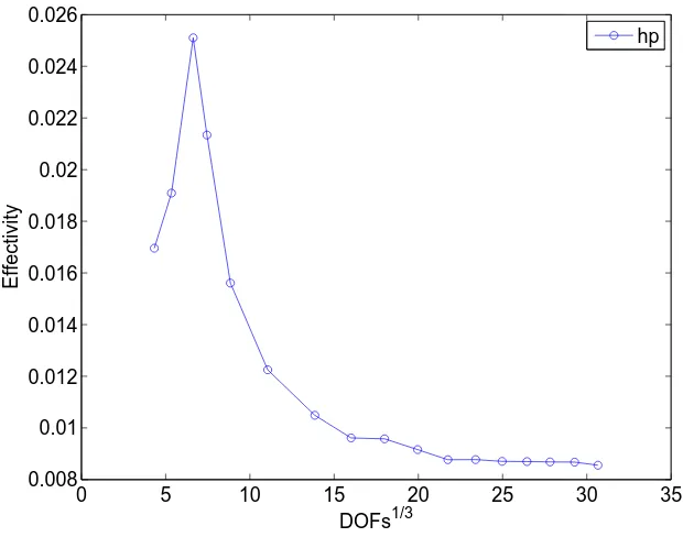
4.1. Unit Triangle. As a simple problem for which the eigenvalues and eigenfunctions are

explic-itly known (cf. [24]), we consider the Type I problem with A=I and Ω is the equilateral triangle

of having unit edge-length. The eigenvalues can be indexed as

λmn=

16π2

9 (m

2_+mn+n2₎

for 0≤m≤n, and we refer interested readers to [24] for explicit descriptions of the eigenfunctions.

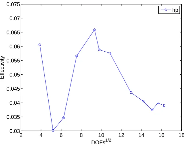
In Figure 1 we plot the total relative errors for the first two eigenvalues, together with the associated error estimates using eitherh-adaptivity orhp-adaptivity. In this case we have obtained

α = 0.3748. In Figure 2 we plot the effectivity quotient for the hp−adaptivity. It is clear that the convergence of thehp-adaptive method is exponential and faster than withh-adaptivity alone. Moreover the error estimator seems to be robust.

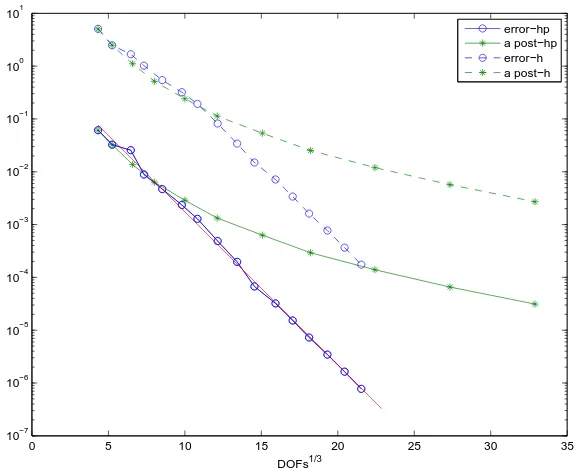
4.2. Triangle with Triangular Hole. Here we again consider a Type I problem with A = I, where Ω is the equilateral triangle having length 2 with an equilateral triangle having edge-length 1/2 removed from its center (see Figure 3).

We now consider the same problem as in the previous example, but in this case, the exact eigenvalues are unknown, so we computed the following reference value for the first eigenvalue, which has multiplicity two, on a very large problem: 3.5591592. This value is accurate at least up to 1e-6.

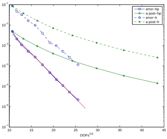
In Figure 4 we plot the relative errors and error estimates for the first two eigenvalues for both

the h-adaptive method and hp-adaptive method. In this case we have obtained α = 0.2539. In

Figure 5 we plot the corresponding values of the effectivity quotient for the hp-adaptive method.

We again see exponential convergence for the hp-adaptive method and clearly only polynomial

0 5 10 15 20 25 10−7

10−6 10−5 10−4 10−3 10−2 10−1 100

DOFs1/2

error−hp a post−hp error−h a post−h

Figure 1. Errors and error estimates. Triangle problem.

2 4 6 8 10 12 14 16 18

0.03 0.035 0.04 0.045 0.05 0.055 0.06 0.065 0.07 0.075

DOFs1/2

Effectivity

hp

Figure 2. Effectivity index. Triangle problem.

4.3. Unit Square. Another standard problem with known eigenvalues is the Neumann Laplacian

on the unit square (Type I, with A=I), for which we have

λmn = (m2+n2)π2 , ψmn= cos(mπx) cos(nπx) , m, n≥0 .

Figure 3. Some domains used in experiments.

10 15 20 25 30 35 40 45

10−7 10−6 10−5 10−4 10−3 10−2 10−1

DOFs1/3

error−hp a post−hp error−h a post−h

Figure 4. Errors and error estimates. Triangle with a hole.

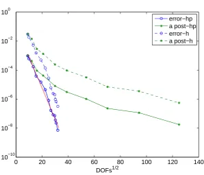
In Figure 6 we plot the relative errors and error estimates for the first two eigenvalues for both

theh-adaptive method andhp-adaptive method. For this example we have obtainedα= 0.2453. In

Figures 7 we plot the corresponding values of the effectivity quotient for the hp-adaptive method.

We again see exponential convergence for the hp-adaptive method and clearly only polynomial

convergence for the h-adaptive method, which is consistent with the theory. In this particular

example the gap between the two adaptive methods is very large, which is understandable in view of the fact that the solutions are smooth, and so increasing the order of the elements reduces the error very rapidly.

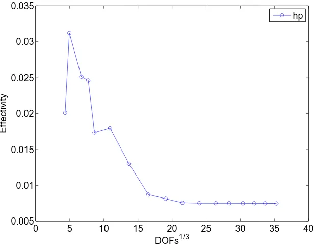
4.4. Unit Square with Discontinuous Diffusion Term. For this Type I problem, Ω is again

10 12 14 16 18 20 22 24 26 0.015

0.02 0.025 0.03 0.035 0.04 0.045 0.05 0.055 0.06

DOFs1/3

Effectivity

hp

Figure 5. Effectivity index. Triangle with a hole.

0 20 40 60 80 100 120 140

10−10 10−8 10−6 10−4 10−2 100

DOFs1/2

error−hp a post−hp error−h a post−h

Figure 6. Errors and error estimates. Square problem.

a = 1 outside the inclusion; and we consider three different values of a inside the inclusion, a=

10, 100, 1000.

In Figures 8, 10 and 12 we plot the total relative errors for the first two eigenvalues, together

with the associated error estimates for the three considered cases for both theh-adaptive method

5 10 15 20 25 30 35 0.022

0.024 0.026 0.028 0.03 0.032 0.034 0.036 0.038

DOFs1/2

Effectivity

hp

Figure 7. Effectivity index. Square problem.

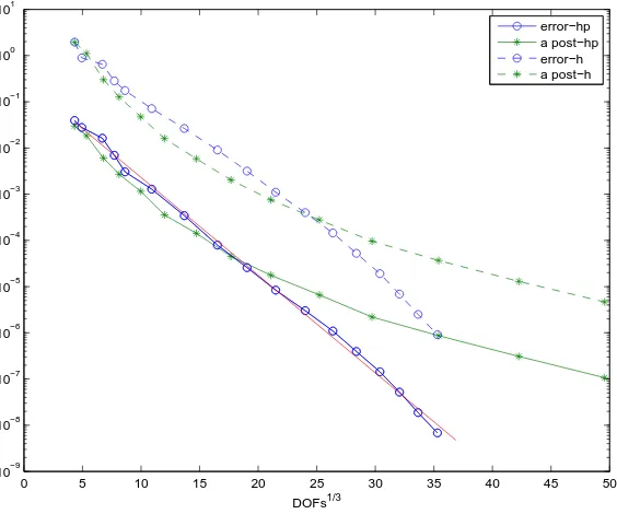
0 5 10 15 20 25 30 35 40 45 50

10−9 10−8 10−7 10−6 10−5 10−4 10−3 10−2 10−1 100 101

DOFs1/3

error−hp a post−hp error−h a post−h

Figure 8. Errors and error estimates. Square problem with a= 10 inside the inclusion.

and hp-adaptive method; and in Figures 9, 11 and 13 we plot the effectivity quotients for the

hp-adaptive method. It is clear that the convergence is exponential in all cases, and that the error estimator is always robust and as it can be seen the effectivity quotient seems to be independent on the jump in value of the coefficientA. Moreover in Figures 14 and 15 we reported the final meshes

0 5 10 15 20 25 30 35 40 0.005

0.01 0.015 0.02 0.025 0.03 0.035

DOFs1/3

Effectivity

hp

Figure 9. Effectivity index. Square problem with a= 10 inside the inclusion.

0 5 10 15 20 25 30 35 40

10−8 10−7 10−6 10−5 10−4 10−3 10−2 10−1 100 101

DOFs1/3

error−hp a post−hp error−h a post−h

Figure 10. Errors and error estimates. Square problem with a= 100 inside the inclusion.

adaptive procedure has automatically heavily refined around the corners of the inclusion, where

the gradient of the eigenfunctions is expected to be unbounded. For such choices of a we have

obtained the following values ofα: 0.2435, 0.2711, and 0.2708, respectively. The fact that these do

not vary much suggest that ourhp-adaptive method is robust with respect to jump discontinuities

0 5 10 15 20 25 30 35 0.008

0.01 0.012 0.014 0.016 0.018 0.02 0.022 0.024 0.026

DOFs1/3

Effectivity

hp

Figure 11. Effectivity index. Square problem with a= 100 inside the inclusion.

0 5 10 15 20 25 30 35 40

10−8 10−7 10−6 10−5 10−4 10−3 10−2 10−1 100 101

DOFs1/3

error−hp a post−hp error−h a post−h

Figure 12. Errors and error estimates. Square problem with a= 1000 inside the inclusion.

all three cases, for a = 10, 100, 1000 are respectively: 21.332601134 (1e-8), 25.635257891 (1e-8) and 26.165986004 (1e-8).

0 5 10 15 20 25 30 35 0.005

0.01 0.015 0.02 0.025

DOFs1/3

Effectivity

hp

Figure 13. Effectivity index. Square problem with a= 1000 inside the inclusion.

Figure 14. Mesh and order of polynomials. Square problem witha= 10 inside the inclusion.

we take Ω as the unit square, partitioned into regionsM1andM2as in Figure 16. We takeA=aI,

Figure 15. Mesh and order of polynomials. Square problem witha= 1000 inside

the inclusion.

0000000

0000000

0000000

0000000

0000000

0000000

0000000

1111111

1111111

1111111

1111111

1111111

1111111

1111111

000000

000000

000000

000000

000000

000000

111111

111111

111111

111111

111111

111111

M2

M2

M1

M1

Figure 16. A modification of the touching squares example of M. Dauge.

with a = 1 in M2, and two different values of a in M1: 5 and 10. Since the exact eigenvalues

are not available, we computed the following three reference values for the first three eigenvalues different from zero: fora= 5 we have 16.683094083 (1e-8), 19.2021789 (1e-6), 27.363024736 (1e-8);

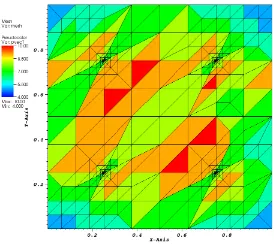
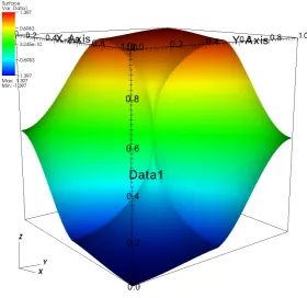
and for a= 10 we have 18.135407487 (1e-8), 25.001324 (1e-5), 28.148296784 (1e-8). In Figure 17

the second eigenvalues for both values ofaare very hard to compute because of such singularities. The presence of these strong singularities has been noticed by the adaptive algorithm, as can be seen in Figure 22 where the region in the center of the domain has been heavily refined.

Figure 17. Eigenfunction of the second eigenvalue different from zero fora= 10.

Convergence and effectivity plots for the first three non-zero eigenvalues are given in Figures

18-19 for a= 5, and in Figures 20-21 for a = 10. When a= 5 we obtain the rate α = 0.3333, and

when a= 10 we obtainα= 0.2542.

4.6. Periodic Problem with Discontinuous Diffusion Term. We consider Type II (periodic)

problem with κ = (0,0), where the “primitive cell” is the unit square with a square inclusion,

precisely as in subsection 4.4. As before, we let A = aI, where a = 1 outside the inclusion and

a= 10 ora= 100 inside the inclusion.

In Figures 23 and 25 we plot the total relative errors for the first two eigenvalues, together with

the associated error estimates for the two considered cases and for both the h-adaptive method

andhp-adaptive method; and in Figure 24 and 26 we plot the effectivity quotients only for thehp -adaptive method. It is clear that the convergence is exponential in both cases using thehp-adaptive

method, and that the error estimator is robust—the vales of α, 0.1752 and 0.1957, respectively,

are pretty close together. The reference values for the first non-zero eigenvalue for a= 10, 100 are respectively: 49.644578674 (2e-8) and 51.146497655 (5e-8).

4.7. Photonic Crystal Example. As last examples we consider the sesquilinear form Bκ in

(2.3), which has applications in nano-optics. For each value of κ the spectrum of Bκ is discrete.

At the same time the eigenvalues form continuous bands when they are seen as function in κ.

0 5 10 15 20 25 30 35 10−7

10−6 10−5 10−4 10−3 10−2 10−1 100 101

DOFs1/3

error−hp a post−hp error−h a post−h

Figure 18. Errors and error estimates. Kellogg problem,a= 5 inM1.

0 5 10 15 20 25

0.004 0.006 0.008 0.01 0.012 0.014 0.016

DOFs1/3

Effectivity

hp

Figure 19. Effectivity index. Kellogg problem,a= 5 inM1.

A typical example of such band structure for a primitive cell with a single inclusion is reported in Figure 27(a). In order to produce accurately the band structure of the crystal it is sufficient

to compute the eigenvalues of Bκ for the values of κ in the reduced Brillouin zone, also called

irreducible Brillouin zone. For sake of clarity we just consider the values of κ on the border of

0 5 10 15 20 25 30 35 10−6

10−5 10−4 10−3 10−2 10−1 100 101 102

DOFs1/3

error−hp a post−hp error−h a post−h

Figure 20. Errors and error estimates. Kellogg problem,a= 10 in M1.

0 5 10 15 20 25

2 3 4 5 6 7 8x 10

−3

DOFs1/3

Effectivity

hp

Figure 21. Effectivity index. Kellogg problem,a= 10 inM1.

minimum and the maximum of each functionλj(κ) delimits a band of the spectrum, and between

bands gaps can sometimes be found. In this example there appears to be a gap between the first and the second band.

Figure 22. Mesh and order of polynomials. Kellogg problem,a= 10 inM1.

A more interesting case is when a compact defect in the periodic structure may create localized eigenvalues in the gaps that correspond to trapped modes. As an example computing the band structure of the supercell we obtain Figure 28(b), where a new narrow band is present in the first gap.

For our examples the domain is the same as in Section 4.4, again with A = aI, and a = 1

outside the inclusion. Inside the inclusion, we takea= 10. Initially we consider two values for the quasi-momentumκ: either (1,1) or (2π,0). For the first of these, operator is positive definite. For the second, it is semi-definite, with Ker(B)∩V ={0}.

In Figures 29 and 31 we plot the relative errors for the second eigenvalues, together with the associated error estimates for the two considered cases and for both theh-adaptive method andhp -adaptive method; and in Figures 30 and 32 we plot the effectivity quotients only for thehp-adaptive

method. It is clear that thehp-adaptive method converges faster than theh-adaptive method and

for the former the values ofαare 0.2194 and 0.1851. The reference values for the eigenvalues in the second band for κ= (1,1), (2π,0) are respectively: 39.745072858 (1e-8) and 49.644578756 (1e-8).

Finally in Figures 33 and 34 we report the convergence of the error for the eigenvalue in the second band for values of κ = (2π−s, s) for the following values of s: 0, 0.1, 0.01, 10e-4, 10e-8, 10e-16. For all values of s, except for s= 0, the corresponding problems have trivial kernels. As can be seen the convergence plots are all very similar, and moreover the effectivity indexes are all in the same range of values for alls. This seems to suggest that the error estimatorεi is robust in

0 10 20 30 40 50 60 10−10

10−8 10−6 10−4 10−2 100 102

DOFs1/3

error−hp a post−hp error−h a post−h

Figure 23. Errors and error estimates. Periodic square problem, a= 10 inside the inclusion.

0 10 20 30 40 50

0 0.02 0.04 0.06 0.08 0.1 0.12 0.14 0.16 0.18 0.2

DOFs1/3

Effectivity

hp

Figure 24. Effectivity index. Periodic square problem,a= 10 inside the inclusion.

5. Concluding Remarks

Thehp-adaptive approach discussed here and in the companion paper [17] provides a robust error theory as well as an efficient, high-order method for eigenvalue and invariant subspace computations. This robustness in theory and practice is with respect to singularities in the eigenfunctions arising

0 5 10 15 20 25 30 35 40 45 10−9

10−8 10−7 10−6 10−5 10−4 10−3 10−2 10−1 100 101

DOFs1/3

error−hp a post−hp error−h a post−h

Figure 25. Errors and error estimates. Periodic square problem, a= 100 inside

the inclusion.

0 5 10 15 20 25 30 35 40

0.01 0.015 0.02 0.025 0.03 0.035 0.04 0.045 0.05

DOFs1/3

Effectivity

hp

Figure 26. Effectivity index. Periodic square problem,a= 100 inside the inclusion.

0 0.2 0.4 0.6 0.8 1 0

0.2 0.4 0.6 0.8 1

x

y

(a) (b)

Figure 27. (a) Structure of the primitive cell. (b) Band structure of the

spec-trum for the periodic crystal with primitive cell as in (a). The first gap has been highlighted in yellow.

0 1 2 3 4 5 0

0.5 1 1.5 2 2.5 3 3.5 4 4.5 5

(a) (b)

Figure 28. (a) Structure of the supercell with a defect in the center. (b) Band structure of the spectrum for the supercell in (a). The first gap has been highlighted in yellow and the newly created trapped band in red.

We point out that, although we have chosen the a posteriori error estimates of Melenk and

Wolmuth [25] in our practical implementation for both “global” error estimates as well as for

selecting elements for refinement, any number of hp a posteriori error estimates for boundary

value problems can be readily “plugged into” our framework with very little change in theory or implementation. For example, one might use a recovery-based approach such as that in [10] or higher-order versions of either [26] or [8]. For each of these approaches an approximate error function is obtained, which gives greater flexibility in how we use it to estimate approximation defects. As can be seen from their definition (via the Courant-Fischer Theorem), the approximation defects

0 10 20 30 40 50 60 10−9

10−8 10−7 10−6 10−5 10−4 10−3 10−2 10−1 100 101

DOFs1/3

error−hp a post−hp error−h a post−h

Figure 29. Errors and error estimates forκ= (1,1).

0 5 10 15 20 25 30 35 40

0.01 0.015 0.02 0.025 0.03 0.035 0.04

DOFs1/3

Effectivity

hp

Figure 30. Effectivity index for κ= (1,1).

are themselves the solutions of a small (m×m) generalized eigenvalue problem—this is discussed

explicitly in [8]. The present approach is based on approximating only the diagonal of the associated

0 10 20 30 40 50 60 10−10

10−8 10−6 10−4 10−2 100 102

DOFs1/3

error−hp a post−hp error−h a post−h

Figure 31. Errors and error estimates forκ= (2π,0).

0 10 20 30 40 50 60 70

0.01 0.02 0.03 0.04 0.05 0.06 0.07 0.08 0.09 0.1

DOFs1/3

Effectivity

hp

Figure 32. Effectivity index for κ= (2π,0).

which permits greater effectivity quotients in the estimates, as was seen in [8] for low-order elements and h-refinement.

Another issue which we plan to address in future work is related to the choice of h- or p

-refinement, a topic which still seems unsettled even for boundary value problems. This choice was made here by estimating local analyticity in the manner of [14]. The complete disconnect between

0 10 20 30 40 50 60 70 10−10

10−8 10−6 10−4 10−2 100 102

DOFs1/3

0.1 0.01 10e−4 10e−8 10e−16 0

Figure 33. Errors and error estimates for κ= (2π−s, s).

0 10 20 30 40 50 60 70

0 0.02 0.04 0.06 0.08 0.1 0.12

DOFs1/3

Effectivity

0.1 0.01 10e−4 10e−8 10e−16 0

Figure 34. Effectivity indexes forκ= (2π−s, s).

the methods used for selecting elements for refinement and the choice how they should be refined is philosophically unappealing, so further efforts will be devoted to developing, if possible, marking and refinement strategies which are more closely related to each other. Any of the “approximate

finite element spaces naturally have a hierarchical structure, anhp-variant of the hierarchical basis approach from [8] is appealing in this regard, and will be pursued further.

Acknowledgement

L. G. was supported by the grant: “Spectral decompositions – numerical methods and applica-tions”, Grant Nr. 037-0372783-2750 of the Croatian MZOS. We would like to thanks Paul Houston and Edward Hall for kind support and very useful discussions.

References

[1] G. Acosta, T. Apel, R. G. Dur´an, and A. L. Lombardi. Anisotropic error estimates for an interpolant defined via moments.Computing, 82:1–9, April 2008.

[2] P. Amestoy, I. Duff, and J.-Y. L’Excellent. Multifrontal parallel distributed symmetric and unsymmetric solvers. Computer Methods in Applied Mechanics and Engineering, 184(2–4):501–520, 2000.

[3] H. Ammari, Y. Capdeboscq, H. Kang, and A. Kozhemyak. Mathematical models and reconstruction methods in magneto-acoustic imaging.European J. Appl. Math., 20(3):303–317, 2009.

[4] H. Ammari, H. Kang, E. Kim, and H. Lee. Vibration testing for anomaly detection.Math. Methods Appl. Sci., 32(7):863–874, 2009.

[5] H. Ammari, H. Kang, and H. Lee. Asymptotic analysis of high-contrast phononic crystals and a criterion for the band-gap opening.Arch. Ration. Mech. Anal., 193(3):679–714, 2009.

[6] M. G. Armentano, C. Padra, R. Rodr´ıguez, and M. Scheble. Anhpfinite element adaptive scheme to solve the Laplace model for fluid-solid vibrations.Comput. Methods Appl. Mech. Engrg., 200(1-4):178–188, 2011. [7] I. Babuˇska and B. Q. Guo. The h-p version of the finite element method for domains with curved boundaries.

SIAM Journal on Numerical Analysis, 25(4):837–861, 1988. ArticleType: research-article / Full publication date: Aug., 1988 / Copyright 1988 Society for Industrial and Applied Mathematics.

[8] R. Bank, L. Grubiˇsi´c, and J. S. Ovall. A framework for robust eigenvalue and eigenvector error estimation and ritz value convergence enhancement.submitted, MPI MSI Leipzig preprint 42/2010, 2010.

[9] R. E. Bank. Hierarchical bases and the finite element method. InActa numerica, 1996, volume 5 ofActa Numer., pages 1–43. Cambridge Univ. Press, Cambridge, 1996.

[10] R. E. Bank, J. Xu, and B. Zheng. Superconvergent derivative recovery for lagrange triangular elements of degree p on unstructured grids.SIAM J. Numer. Anal., submitted.

[11] T. Betcke and L. N. Trefethen. Reviving the method of particular solutions.SIAM Rev., 47(3):469–491 (elec-tronic), 2005.

[12] M. Blumenfeld. Interface-Eigenwertprobleme auf polaren Gittern.Z. Angew. Math. Mech., 64(5):266–268, 1984. [13] M. Blumenfeld. The regularity of interface-problems on corner-regions. InSingularities and constructive methods for their treatment (Oberwolfach, 1983), volume 1121 ofLecture Notes in Math., pages 38–54. Springer, Berlin, 1985.

[14] T. Eibner and J. Melenk. An adaptive strategy for hp-fem based on testing for analyticity.Comp. Mech., 39:575– 595, 2007.

[15] S. C. Eisenstat. On the rate of convergence of the Bergman-Vekua method for the numerical solution of elliptic boundary value problems.SIAM J. Numer. Anal., 11:654–680, 1974.

[16] S. Giani and I. Graham. Adaptive finite element methods for computing band gaps in photonic crystals. Nu-merische Mathematik, to appear.

[17] S. Giani, L. Grubiˇsi´c, and J. Ovall. Reliablea-posteriori error estimators forhp-adaptive finite element approx-imations of eigenvalue/eigenvector problems. Nothingam ePrints, http://eprints.nottingham.ac.uk/, 2011. [18] S. Giani, L. Grubiˇsi´c, and J. Ovall. Benchmark results for testing adaptive finite element eigenvalue procedures.

Applied Numerical Mathematics, 62(2):121–140, 2012.

[19] L. Grubiˇsi´c. On eigenvalue and eigenvector estimates for nonnegative definite operators.SIAM J. Matrix Anal. Appl., 28(4):1097–1125 (electronic), 2006.

[20] L. Grubiˇsi´c. Relative convergence estimates for the spectral asymptotic in the large coupling limit. Integral Equations Operator Theory, 65(1):51–81, 2009.

[21] L. Grubiˇsi´c and J. S. Ovall. On estimators for eigenvalue/eigenvector approximations.Math. Comp., 78:739–770, 2009.

[22] P. Houston and E. S¨uli. A note on the design of hp-adaptive finite element methods for elliptic partial differential equations.Computer Methods in Applied Mechanics and Engineering, 194(2-5):229–243, Feb. 2005.

[23] R. B. Kellogg. On the Poisson equation with intersecting interfaces.Applicable Anal., 4:101–129, 1974/75. Col-lection of articles dedicated to Nikolai Ivanovich Muskhelishvili.

[24] B. J. McCartin. Eigenstructure of the equilateral triangle. II. The Neumann problem. Math. Probl. Eng., 8(6):517–539, 2002.

[25] J. M. Melenk and B. I. Wohlmuth. On residual-based a posteriori error estimation in hp-FEM.Adv. Comput. Math., 15(1-4):311–331 (2002), 2001. A posteriori error estimation and adaptive computational methods. [26] A. Naga and Z. Zhang. Function value recovery and its application in eigenvalue problems. SIAM J. Numer.

Anal., to appear.

[27] J. Weidmann. Stetige Abh¨angigkeit der Eigenwerte und Eigenfunktionen elliptischer Differentialoperatoren vom Gebiet.Math. Scand., 54(1):51–69, 1984.

School of Mathematical Sciences University of Nottingham , University Park, Nottingham, NG7 2RD, United Kingdom

E-mail address: [email protected]

University of Zagreb, Department of Mathematics, Bijeniˇcka 30, 10000 Zagreb, Croatia E-mail address: [email protected]

University of Kentucky, Department of Mathematics, Patterson Office Tower 761, Lexington, KY 40506-0027, USA