C
2010. The American Astronomical Society. All rights reserved. Printed in the U.S.A.
STRUCTURE FORMATION BY FIFTH FORCE: POWER SPECTRUM FROM
N
-BODY SIMULATIONS
Hongsheng Zhao1,2, Andrea V. Macci `o3, Baojiu Li4,5, Henk Hoekstra2, and Martin Feix1
1SUPA, School of Physics and Astronomy, University of St. Andrews, KY16 9SS, UK 2Leiden University, Leiden Observatory, Niels-Borhweg 2, 2333CA, Leiden, The Netherlands
3Max-Planck-Institut f¨ur Astronomie, K¨onigstuhl 17, 69117 Heidelberg, Germany 4DAMPT, Centre for Mathematical Sciences, University of Cambridge, CB3 0WA, UK 5Kavli Institute for Cosmology Cambridge, Madingley Road, Cambridge CB3 0HA, UK
Received 2009 October 15; accepted 2010 February 8; published 2010 March 17
ABSTRACT
We lay out the framework to numerically study nonlinear structure formation in the context of scalar-field-coupled cold dark matter models (ϕCDM models) where the scalar field ϕ serves as dynamical dark energy. Adopting parameters for the scalar field that leave negligible effects on the cosmic microwave background (CMB) spectrum, we generate the initial conditions for ourN-body simulations. The simulations follow the spatial distributions of dark matter and the scalar field, solving their equations of motion using a multilevel adaptive grid technique. We show that the spatial configuration of the scalar field depends sensitively on the local density field. The ϕCDM model differs from standard ΛCDM at small scales with observable modifications of, e.g., the mass function of halos as well as the matter power spectrum. Nevertheless, the predictions of both models for the Hubble expansion and the CMB spectrum are virtually indistinguishable. Hence, galaxy cluster counts and weak lensing observations, which probe structure formation at small scales, are needed to falsify this class of models.
Key words: cosmology: theory – methods: numerical
Online-only material:color figures
1. INTRODUCTION
The origin and nature of dark energy (Copeland et al.2006) is one of the most difficult challenges facing physicists and cosmologists at the present time. Among all the proposed models to tackle this problem, the introduction of a scalar field is perhaps the most popular. The scalar field, denoted byϕ, should have no coupling to normal matter to be consistent with stringent constraints from experiments (Will 2006, and references therein), but could couple to the dark matter, therefore producing a fifth force between dark matter particles. This idea has gained a lot of interest in recent years because dark matter physics are unknown, and such a coupling could alleviate the coincidence problem of dark energy (e.g., Amendola 2000; Chiba2001; Chimento et al.2003). Furthermore, it is commonly predicted by low-energy effective theories derived from a more fundamental theory. A specific and interesting possibility is the chameleon mechanism (Khoury & Weltman2004; Mota & Shaw2006), by virtue of which the scalar field acquires a large mass in high-density regions and thus the fifth force becomes undetectable on short ranges, thus also evading constraints from the large-scale cosmic microwave background (CMB). Indeed, at the linear perturbation level, there have been a lot of studies about the coupled scalar field andf(R) gravity models (e.g., Li & Barrow2007; Hu & Sawicki2007).
Nevertheless, little is known about these models on nonlinear scales. It is well known that the matter distribution at late times, i.e.,z2 for cluster scales, evolves in a nonlinear way, making the behavior of the scalar field more complex and the linear analysis insufficient to produce accurate results that can be confronted with observations. For the latter purpose, the best way forward is to perform fullN-body simulations (Bertschinger
1998) to evolve the individual particles step by step.
N-body simulations including scalar fields and related models have been performed before (Linder & Jenkins2003; Mainini et al.2003; Macci`o et al.2004; Springel & Farrar2007; Kesden
& Kamionkowski 2006a,2006b; Farrar & Rosen2007; Baldi et al.2010; Oyaizu2008; Keselman et al.2010; Li & Zhao2009). For example, in the work of Macci`o et al. (2004), the simulations included several effects due to the coupling between dark energy and dark matter (e.g., modified gravitational constant, an extra dragging term in Newton’s equations and time variable dark matter particle masses), but did not consider a spatial variation of the dark energy scalar field. The more complete simulation of the scalar field by Li & Zhao (2009) shows that this approximation is only good for a limited choice of parameters and the scalar field potential. Here we extend the work of Li & Zhao (2009).
This Letter is organized as follows: in Section 2, we shall briefly review the general equations of motion for the coupled scalar field model introduced in Li & Zhao (2009), and present our specific choices of the coupling function and the scalar field potential. In Section3, we describe the formulae and the algorithm of theN-body simulation, analyze the results of our coupled scalar fieldN-body simulations, compare it with that of the standardΛCDM model, and explain the physical origin of the new features. Finally, we conclude and discuss observational implications in Section4.
2. THE COUPLED SCALAR FIELD MODEL
2.1. The Model
All properties of our coupled scalar field model can be derived from minimizing the action associated with the following Lagrangian density (the indexaruns from 0 to 3):
L=
R 2 −
1 2∇
aϕ∇
aϕ+Veff(ϕ)
, (1)
which includes the Ricci scalarR, and a dimensionless scalar fieldϕwith a kinetic and an effective potential term. The latter is given by
Veff(ϕ)≡V(ϕ)−κ(ϕ)LCDM, (2)
Veff(ϕ)≈Λ0ϕ−μ+ 8π G(1 +γ ϕ)ρCDM, (4)
the meaning of this particular parameterization can be under-stood as follows: as the scalar field ϕ tends to minimize the effective potential, the potential termΛ0ϕ−μ and the coupling (1 + γ ϕ) to the cold dark matter (CDM) density (ρCDM ∼
−LCDMin the nonrelativistic, weak-field limit) lead to compet-ing effects, favorcompet-ing smaller and larger values ofϕ, respectively.6 The balance of these two effects, minimizing the effective po-tentialVeff, is controlled by the two dimensionless parameters μandγ: μis very small and controls the time when the ef-fect of the scalar field (mainly exerting the finite-ranged fifth force on dark matter particles on galaxy cluster scales) becomes important for cosmology whileγ determines how large it will ultimately be (Li & Zhao2009). More specifically, the scalar field equation of motion is
ϕ+∂V(ϕ)
∂ϕ +ρCDM8π Gγexp(γ ϕ)=0. (5)
Einstein’s equations can be expressed as
1
8π GGab =exp(γ ϕ)ρCDMuaub+T ϕ
ab, (6)
whereGab is the Einstein tensor, and the right-hand side is the
energy–momentum tensor of the scalar field and CDM with a four-velocityua; the scalar field is given by
8π GTabϕ = ∇aϕ∇bϕ−gab
1 2∇cϕ∇
cϕ−V (ϕ)
. (7)
Note that the energy–momentum tensors for the scalar fieldϕ and the dark matter are not individually conserved due to their coupling, whereas their sum is.
Equations (5) and (6) summarize all the physics that will be used in our analysis. An immediate application is the prediction of a uniform Hubble expansion. The model’s expansion is completely indistinguishable fromΛCDM for values of γ ∼
O(1) andμ1; the actual difference is on the order ofO(μ). Basically, this is due to the large enough scalar’s mass, forcing the field near the potential minimum, which itself is almost time independent forμ1. A quantitative explanation is given in Li & Zhao (2009). We now proceed to break the degeneracy via nonlinear clustering.
2.2. The Nonrelativistic Equations
The first step toward a numerical simulation is to simplify the relevant equations of motion in the nonrelativistic and quasi-static limit (in the sense that the time derivatives can be safely neglected compared with the spatial derivatives).
6 The dark matter LagrangianL
CDMspecifies the geodesic flow for many
pointlike particles of four-velocityuaand densityρCDM.
Finally, the equations of motion of the dark matter particles are also modified as
dx
dt =
p
a2, (10)
dp
dt = − 1
a∇xΦ−γ∇xϕ, (11) where the canonical momentum conjugate to the comoving coordinatesxisp=a2x˙. Note that the two terms on the right-hand side of Equation (11) correspond to gravity and fifth force, respectively (Li & Zhao2009). The scalar fieldϕis on the order of magnitude ofμ, comparable to the dimensionless potentialΦ. Equations (8)–(11) are used in the code to evaluate the forces on the dark matter particles and to evolve their positions and momenta in time.
The validity and limitation of the approximation present in the above equations, in particular neglecting the time derivatives, have been extensively discussed in Li & Zhao (2009). We emphasize that these approximations do not hold in the linear regime where the scalar field’s time dependence is essential for structure growth. However, such terms have indeed been shown to be negligible on scales much smaller than the horizon scale (Li & Zhao2009; Oyaizu2008). To make our predictions more quantitative and rigorous compared to previous analyses (Macci`o et al.2004; Kesden & Kamionkowski2006a,2006b; Farrar & Rosen 2007), we now analyze the first N-body simulations in the above framework. Considering the linear regime, Li & Zhao (2009) have already been able to constrain the parametersμandγ to a fairly narrow range. Here we set γ on the order of unity to force a significant ratio of the fifth force to gravity (∼2γ), and explore the range 10−7 μ 10−5, covering 3 orders of magnitude. Restricting ourselves to the above should suffice as the model is either essentially indistinguishable from ΛCDM or deviates too much from it (already at the linear level) beyond this parameter space, thus being of no further interest (Li & Zhao2009).
3. NONLINEAR STRUCTURE FORMATION
In this section, we present some results of the firstN-body runs and describe the qualitative behavior of the coupled scalar field model.
3.1. The N-body Code
We adapt the multi-level adaptive particle mesh (MLAPM) code (Knebe et al. 2001) to include the scalar field, and its coupling to the dark matterN-body particles. One benefit of the
7 The notation∂2
x = − ∇x2=∂x2+∂y2+∂z2is defined with respect to the comoving coordinatexsuch that∇x=a∇r, whereais the usual scale factor of the universe. In the following,ϕ¯andρ¯CDMdenote the background values of
ϕandρCDM, respectively. Although we have used the approximation
ρCDMexp(γ ϕ)∼ρCDMfor a simpler presentation, we keep the factor exp(γ ϕ)
Figure 1.Overdensity fields atz = 0 for theϕCDM model with γ = 1,
μ=10−5(left) and theΛCDM model (right). The former has developed more
small-scale structure within the void.
(A color version of this figure is available in the online journal.)
adaptive scheme is that the majority of computing resources is dedicated to few high-density regions to ensure higher resolution, which is desirable since we expect the behavior of the scalar field to be more complex there.
The main modifications to the MLAPM code for our model are as follows:
1. We have added a parallel solver for the scalar field based on Equation (8). The solver uses a similar nonlinear Gauss–Seidel method (Briggs et al.2000; Press et al.1992) and the same criterion for convergence as the Poisson solver. 2. The resulting value forϕof the first step is used to calculate the local mass density of the scalar field and thus the source term for Poisson’s equation, which is solved using a fast Fourier transform to obtain the local gravitational potential
Φ(cf. Equation (9)).
3. The fifth force is obtained by differentiating ϕ, and the gravitational force is calculated by differentiatingΦ, as in Equations (10) and (11).
4. The momenta and positions of particles are then updated, taking into account both gravity and the fifth force, just as in normalN-body codes.
More technical details on the code, as well as how Equations (8)–(11) are incorporated into MLAPM using its own internal units, have been given in Li & Zhao (2009) and will not be presented here.
3.2. Numerical Results from the N-body Runs
We have performed six runs of the modified code with parametersγ =0.5,1 andμ=10−5,10−6,10−7, respectively. For all these runs, there are 1283 dark matter particles, and the simulation box size is chosen as B = 64h−1Mpc, with
[image:3.612.46.290.55.185.2]h being the usual dimensionless Hubble parameter and 128 domain grid cells in each direction. We assume a ΛCDM background cosmology which is a very good approximation for μ 1 (Li & Zhao2009); in addition, we adopt present values for the fractional energy densities of dark matter and dark energy,ΩCDM =0.28 andΩΛ =0.72, and the normalization of the power spectrum is chosen asσ8 = 0.88. Note that the simulation does only take dark matter into account, baryons will be added in a forthcoming work to study the bias effect caused by the dark matter coupling. Given these parameters, the mass and spatial resolution of the simulation are 9.71×10⁹M and∼23.44h−1kpc (for the most refined regions), respectively. This spatial resolution in high-density regions is necessary and sufficient to precisely probe the scalar field in regions where the fifth force is considerably short-ranged.
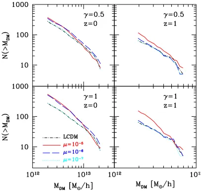
Figure 2.Mass functions forγ =0.5 (upper panels) andγ =1 (lower panels) for different values ofμatz=0 andz=1. TheΛCDM mass function is also plotted as a (black) dot-dashed curve for comparison.
(A color version of this figure is available in the online journal.)
All simulations started at redshiftz=49. In principle, mod-ified initial conditions, i.e., the initial displacements and veloc-ities of particles which are obtained from a given linear matter power spectrum, need to be generated for the coupled scalar field model because the Zel’dovich approximation (Efstathiou et al. 1985) is also affected by the scalar field coupling. In practice, however, we find that the effect on the linear matter power spectrum at this high redshift is negligible (O(10−4)) for our choice of the parametersγ andμ. Thus we simply use the ΛCDM initial displacements/velocities for the CDM par-ticles in our simulations, which are generated using GRAFIC (Bertschinger 1995), again usingΩCDM = 0.28, ΩΛ = 0.72, andσ8=0.88. An example of the final density field at redshift z = 0 is shown in Figure1 for comparison with theΛCDM simulation.
We look for all virialized isolated halos within our compu-tational volume using a spherical overdensity algorithm. For this purpose, we employ a time-varying virial density contrast which is determined using the fitting formula presented in Main-ini et al. (2003), and adopt the same virial density contrast for all models. In addition, we include all haloes with more than 200 particles into the halo catalog (see Macci`o et al.2008for further details on our halo finding algorithm). Power spectra have been computed through a (fast) Fourier transform of the matter density field, computed on a regular gridNG×NG×NG from the particle distribution via a cloud-in-cell algorithm (see Casarini et al.2009). We setNG=256 which gives a maximum mode ofk≈20hMpc−1well above the simulation resolution. In Figure2, we show the mass functions for the runs with γ =1.0,0.5, andμ=10−5,10−6,10−7and the fiducialΛCDM simulation at two output redshiftsz=1 and 0. The nonlinear matter power spectra of these models are displayed in Figures3
and4, respectively.
3.3. Interpretation of the Results
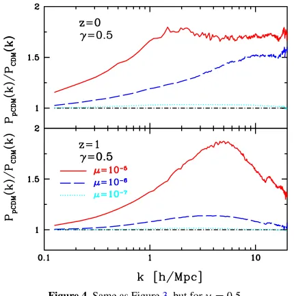
Figure 3.Ratios of calculated nonlinear matter power spectra forγ =1 and
μ = 10−5 (solid), 10−6 (dashed), and 10−7 (dotted) as well as for that of
ΛCDM. Shown are results for two redshifts,z=1,0. At large scales (smallk), the curves converge to the horizontal curves (identical to 1, dot-dashed). Note that, using analytic results, the difference is expected to be small on both large and very small scales, and decreases at higher redshift. Error bars of future lensing observations are likely small enough to detect any deviation fromΛCDM on intermediate scales (k=0.1–10hMpc−1) at a 30% level.
(A color version of this figure is available in the online journal.)
essentially leads to an increase in the effective gravitational constant which governs structure formation (Macci`o et al.2004). Li & Zhao (2009) have shown that for certain regions of parameter space and specific choices of the potential, this is indeed a good approximation. Mathematically, this corresponds to neglecting the source terms starting withΛ0in Equations (8) and (9); hence the fifth forceγ∇ϕ is about a factor 2γ2 times the gravitational force∇Φ/a.
In another situation, when the scalar field has a very steep potential,mϕ depends sensitively on the local matter density (Khoury & Weltman 2004) so that it almost resides at the minimum of its effective potential,
Veff(ϕ)=V(ϕ) + 8π GρCDMexp(γ ϕ), (12)
throughout space, i.e., ϕ ∼ Λ0μ/(8π GρCDM). This is known as the chameleon effect whose direct consequence is that in a high-density environment,m2
ϕgets very heavy,
m2ϕ=∂2Veff/∂ϕ2=Λ0μ(1 +μ)ϕ−μ−2∝μ−1ρCDM−2 , (13)
and the fifth force becomes very short-ranged, with its effect being suppressed due toγ∇φ ∝ γ μ∇ρCDM−1 . In general, the smaller μ is, and/or the larger γ , ρCDM are, the heavier mϕ becomes and thus the stronger the chameleon effect will be. Furthermore, since the value ofϕinside a region also depends on its boundary condition, which in our case matches the background ϕ¯ asymptotically, we see that a smaller ϕ¯ leads to a smallerϕ and a heavier mϕ, and therefore to a stronger chameleon effect.
There are several interesting features in Figure2which can be understood schematically. First of all, our models produce more halos within the considered mass range thanΛCDM due to the enhancing effect of the fifth force. Second, a smaller μ means that the fifth force is more severely suppressed by the chameleon effect, and thus causes a small deviation from
Figure 4.Same as Figure3, but forγ =0.5. (A color version of this figure is available in the online journal.)
ΛCDM. Thirdly, a largerρCDM also means that the fifth force is more severely suppressed, and this is why at high redshifts the deviation fromΛCDM (for the sameγ andμ) is smaller. Fourthly, the influence of the parameterγis more complicated: a larger γ will strengthen the chameleon effect, tending to suppress the fifth force, but at the same time it increases the magnitude of the fifth force. In cases where the chameleon effect is weak (e.g.,μ=10−5), however, we do see that a larger γ leads to larger deviations fromΛCDM.
Also note that the deviation from theΛCDM mass function is more significant toward the low-mass end. To understand why this is the case, consider a mass range [M0, M0+ΔM]. At a certain redshift, some halos which should have been in this range inΛCDM indeed fall into the mass range (M0+ΔM,∞) in our model as the fifth force accelerates the formation of structures (this tends to reduce the number of halos with mass> M0as two halos which are separated inΛCDM merge into one here), while some halos which should have been in the mass range< M0in
ΛCDM actually fall in the mass range [M0, M0+ΔM] in our model (this increases the number of halos with mass > M0). This effect is weaker for the largest halos because of competing effects due to merging of small halos. As the mass increases, the difference between the mass functions of the two models narrows down.
In the matter power spectrum, we see something similar: smallerμand largerρCDM (higher redshift) severely suppress the fifth force and lead to smaller deviations from ΛCDM; increasingγ strengthens the fifth force, thereby causing large deviations from ΛCDM. Interestingly, the deviation becomes largest on intermediate scales: large scales are beyond the probe of the fifth force, and thus not significantly affected, while the density on small scales is high and the fifth force is suppressed.
4. CONCLUSION
[image:4.612.337.552.54.270.2]On these scales, the matter power spectrum is significantly in-creased compared to that ofΛCDM. Observationally, this would most likely appear as a change ofσ8on the order of 15%–20% for models withγ =0.5–1 andμ=10−6(see Figure2). Any variation ofσ8seems to be lower than 30% for current lensing measurements such as the Canada–France–Hawaii Telescope Legacy Survey (e.g., Hoekstra et al.2006; Figure 11 of Fu et al.
2008) over a rather limited range; however, future surveys, such as the Kilo-Degree Survey, will be able to measure the scale dependence within the rangek = 0.1–10h Mpc−1, where the deviation of the models fromΛCDM is maximal.
This work has been performed within the HPC-EUROPA project, with the support of the European Community Research Infrastructure Action under the FP8 “Structuring the European Research Area” Programme. We thank Simon-Porteges Zwart and Marco Baldi for discussions. H. Zhao is thankful for finan-cial support from the Dutch NWO visitorship No.040.11.089 to Henk Hoekstra, B. Li acknowledges financial support from a UK Overseas Research Studentship, the Cambridge Overseas Trust and Queens’ College Cambridge. M. Feix is supported by a scholarship from the Scottish Universities Physics Alliance (SUPA).
REFERENCES
Amendola, L. 2000,Phys. Rev. D,62, 043511
Baldi, M., Pettorino, V., Robbers, G., & Springel, V. 2010, MNRAS, in press (arXiv:0812.3901 [astro-ph])
Bertschinger, E. 1995, arXiv:astro-ph/9506070
Bertschinger, E. 1998,ARA&A,36, 599
Briggs, W. L., Henson, V. E., & McCormick, S. F. 2000, A Multigrid Tutorial (2nd ed.; Philadelphia, PA: SIAM)
Casarini, L., Macci`o, A. V., & Bonometto, S. A. 2009,J. Cosmol. Astropart. Phys.,3, 14
Chiba, T. 2001,Phys. Rev. D,64, 103503
Chimento, L. P., Jakubi, A. S., Pav´on, D., & Zimdahl, W. 2003,Phys. Rev. D,
67, 083513
Copeland, E. J., Sami, M., & Tsujikawa, S. 2006,Int. J. Mod. Phys. D,15, 1753
Efstathiou, G., Davis, M., White, S. D. M., & Frenk, C. S. 1985,ApJS,57, 241
Farrar, G. R., & Rosen, R. A. 2007,Phys. Rev. Lett.,98, 171302
Fu, L., et al. 2008,A&A,479, 9
Hoekstra, H., et al. 2006,ApJ,647, 116
Hu, W., & Sawicki, I. 2007,Phys. Rev. D,76, 064004
Kesden, M., & Kamionkowski, M. 2006a,Phys. Rev. Lett.,97, 131303
Kesden, M., & Kamionkowski, M. 2006b,Phys. Rev. D,74, 083007
Keselman, J. A., Nusser, A., & Peebles, P. J. E. 2010, Phys. Rev. D, in press Khoury, J., & Weltman, A. 2004,Phys. Rev. Lett.,93, 171104
Knebe, A., Green, A., & Binney, J. 2001,MNRAS,325, 845
Li, B., & Barrow, J. D. 2007,Phys. Rev. D,75, 084010
Li, B., & Zhao, H. 2009,Phys. Rev. D,80, 044027
Linder, E. V., & Jenkins, A. 2003,MNRAS,346, 573
Macci`o, A. V., Dutton, A. A., & van den Bosch, F. C. 2008,MNRAS,391, 1940
Macci`o, A. V., Quercellini, C., Mainini, R., Amendola, L., & Bonometto, S. A. 2004,Phys. Rev. D,69, 123516
Mainini, R., Macci`o, A. V., Bonometto, S. A., & Klypin, A. 2003,ApJ,599, 24
Mota, D. F., & Shaw, D. J. 2006,Phys. Rev. Lett.,97, 151102
Oyaizu, H. 2008,Phys. Rev. D,78, 123523
Press, W. H., Teukolsky, S., Vetterling, W. T., & Flannery, B. P. 1992, Numerical Recipes in C. The Art of Scientific Computing (2nd ed.; Cambridge: Cambridge Univ. Press)
Springel, V., & Farrar, G. R. 2007,MNRAS,380, 911