Munich Personal RePEc Archive
ARIMA modeling and forecasting of
inflation in Egypt (1960-2017)
NYONI, THABANI
University of Zimbabwe
25 February 2019
ARIMA Modeling and Forecasting of Inflation in Egypt (1960 – 2017)
Nyoni, Thabani
Department of Economics
University of Zimbabwe
Harare, Zimbabwe
Email: [email protected]
ABSTRACT
This research uses annual time series data on inflation rates in Egypt from 1960 to 2017, to model and forecast inflation using ARIMA models. Diagnostic tests indicate that E is I(1). The study presents the ARIMA (0, 1, 1). The diagnostic tests further imply that the presented optimal ARIMA (0, 1, 1) model is stable and acceptable for predicting inflation in Egypt. The results of the study apparently show that E will be approximately 23.3% over the out-of-sample forecast period. The CBE is expected to continue tightening Egypt’s monetary policy in order to restore price stability.
Key Words: Egypt , Forecasting, Inflation
JEL Codes: C53, E31, E37, E47
INTRODUCTION
Inflation is the sustained increase in the general level of prices and services over time (Blanchard, 2000). The monetary policy objective of the Central Bank of Egypt (CBE) is achieving low rates of inflation essential for sustaining high investment and growth rates as well as maintaining confidence in the Egyptian economy (Hosny, 2016). Low inflation is a key for macroeconomic stability as evidenced by many country experiences, since high inflation in general hurt macroeconomic stability mainly through lower domestic savings by deeply negative real interest rates, lower capital accumulation due to increased uncertainty, and real appreciation of the exchange rate reflecting widened inflation differentials against trade partners (Moriyama, 2011). To prevent the aforementioned undesirable outcomes of price instability, central banks require proper understanding of the future path of inflation to anchor expectations and ensure policy credibility; the key aspects of an effective monetary policy transmission mechanism (King, 2005). Inflation forecasts and projections are also often at the heart of economic policy decision-making, as is the case for monetary policy, which in most industrialized economies is mandated to maintain price stability over the medium term (Buelens, 2012). Economic agents, private and public alike; monitor closely the evolution of prices in the economy, in order to make decisions that allow them to optimize the use of their resources (Hector & Valle, 2002). To avoid adjusting policy and models by not using an inflation rate prediction can result in imprecise investment and saving decisions, potentially leading to economic instability (Enke & Mehdiyev, 2014). In this study, we seek to model and forecast inflation in Egypt using ARIMA models. The study is envisaged to assist the CBE in restoring macroeconomic stability in Egypt.
Nyoni (2018) studied inflation in Zimbabwe using GARCH models with a data set ranging over the period July 2009 to July 2018 and established that there is evidence of volatility persistence for Zimbabwe’s monthly inflation data. Once gain, Nyoni (2018) modeled inflation in Kenya using ARIMA and GARCH models and relied on annual time series data over the period 1960 – 2017 and found out that the ARIMA (2, 2, 1) model, the ARIMA (1, 2, 0) model and the AR (1)
– GARCH (1, 1) model are good models that can be used to forecast inflation in Kenya. Nyoni & Nathaniel (2019), based on ARMA, ARIMA and GARCH models; studied inflation in Nigeria using time series data on inflation rates from 1960 to 2016 and found out that the ARMA (1, 0, 2) model is the best model for forecasting inflation rates in Nigeria.
MATERIALS & METHODS
Box – Jenkins ARIMA Models
One of the methods that are commonly used for forecasting time series data is the Autoregressive Integrated Moving Average (ARIMA) (Box & Jenkins, 1976; Brocwell & Davis, 2002; Chatfield, 2004; Wei, 2006; Cryer & Chan, 2008). For the purpose of forecasting inflation rate in Egypt, ARIMA models were specified and estimated. If the sequence ∆dEt satisfies an ARMA (p, q) process; then the sequence of Et also satisfies the ARIMA (p, d, q) process such that:
∆𝑑𝐸
𝑡 = ∑ 𝛽𝑖∆𝑑𝐸𝑡−𝑖+ 𝑝
𝑖=1
∑ 𝛼𝑖𝜇𝑡−𝑖 𝑞
𝑖=1
+ 𝜇𝑡… … … . … … … … . … … . [1]
which we can also re – write as:
∆𝑑𝐸
𝑡 = ∑ 𝛽𝑖∆𝑑𝐿𝑖𝐸𝑡 𝑝
𝑖=1
+ ∑ 𝛼𝑖𝐿𝑖𝜇𝑡 𝑞
𝑖=1
+ 𝜇𝑡… … … . . … … … . … … … [2]
where ∆ is the difference operator, vector β ϵⱤp
and ɑ ϵⱤq.
The Box – Jenkins Methodology
The first step towards model selection is to difference the series in order to achieve stationarity. Once this process is over, the researcher will then examine the correlogram in order to decide on the appropriate orders of the AR and MA components. It is important to highlight the fact that this procedure (of choosing the AR and MA components) is biased towards the use of personal judgement because there are no clear – cut rules on how to decide on the appropriate AR and MA components. Therefore, experience plays a pivotal role in this regard. The next step is the estimation of the tentative model, after which diagnostic testing shall follow. Diagnostic checking is usually done by generating the set of residuals and testing whether they satisfy the characteristics of a white noise process. If not, there would be need for model re – specification and repetition of the same process; this time from the second stage. The process may go on and on until an appropriate model is identified (Nyoni, 2018).
Data Collection
Diagnostic Tests & Model Evaluation
[image:4.612.79.552.140.394.2]Stationarity Tests: Graphical Analysis
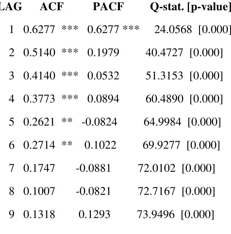
Figure 1
The Correlogram in Levels
Autocorrelation function for EGINF ***, **, * indicate significance at the 1%, 5%, 10% levels.
Table 1
LAG ACF PACF Q-stat. [p-value]
1 0.6277 *** 0.6277 *** 24.0568 [0.000]
2 0.5140 *** 0.1979 40.4727 [0.000]
3 0.4140 *** 0.0532 51.3153 [0.000]
4 0.3773 *** 0.0894 60.4890 [0.000]
5 0.2621 ** -0.0824 64.9984 [0.000]
6 0.2714 ** 0.1022 69.9277 [0.000]
7 0.1747 -0.0881 72.0102 [0.000]
8 0.1007 -0.0821 72.7167 [0.000]
9 0.1318 0.1293 73.9496 [0.000] -5
0 5 10 15 20 25 30
[image:4.612.75.313.485.726.2]10 -0.0852 -0.3795 *** 74.4762 [0.000]
11 -0.1246 0.0165 75.6259 [0.000]
The ADF Test in Levels
Table 2: Levels-intercept
Variable ADF Statistic Probability Critical Values Conclusion
E -1.910422 0.3253 -3.552666 @1% Non-stationary
-2.914517 @5% Non-stationary -2.595033 @10% Non-stationary Table 3: Levels-trend & intercept
Variable ADF Statistic Probability Critical Values Conclusion
E -2.091735 0.5389 -4.130526 @1% Non-stationary
-3.492149 @5% Non-stationary -3.174802 @10% Non-stationary Table 4: without intercept and trend & intercept
Variable ADF Statistic Probability Critical Values Conclusion
E -0.244355 0.5937 -2.606911 @1% Non-stationary
[image:5.612.65.545.164.400.2]-1.946764 @5% Non-stationary -1.613062 @10% Non-stationary Figure 1 and tables 1 – 4 show that E is non-stationary in levels.
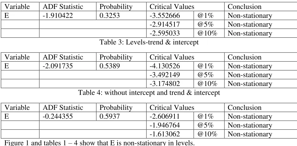
The Correlogram (at 1st Differences)
[image:5.612.75.312.496.708.2]Autocorrelation function for d_EGINF ***, **, * indicate significance at the 1%, 5%, 10% levels. s
Table 5
LAG ACF PACF Q-stat. [p-value]
1 -0.2563 * -0.2563 * 3.9442 [0.047]
2 -0.0077 -0.0785 3.9478 [0.139]
3 -0.0898 -0.1207 4.4501 [0.217]
4 0.1661 0.1187 6.1999 [0.185]
5 -0.1207 -0.0606 7.1419 [0.210]
6 0.1119 0.0825 7.9681 [0.240]
7 -0.1137 -0.0597 8.8378 [0.265]
9 0.3828 *** 0.3410 ** 22.2938 [0.008]
10 -0.1994 -0.1748 25.1383 [0.005]
11 0.0999 0.1291 25.8684 [0.007]
ADF Test in 1st Differences
Table 6: 1st Difference-intercept
Variable ADF Statistic Probability Critical Values Conclusion
E -9.161287 0.0000 -3.552666 @1% Stationary
[image:6.612.64.547.187.433.2]-2.914517 @5% Stationary -2.595033 @10% Stationary Table 7: 1st Difference-trend & intercept
Variable ADF Statistic Probability Critical Values Conclusion
E -9.074184 0.0000 -4.130526 @1% Stationary
-3.492149 @5% Stationary -3.174802 @10% Stationary Table 8: 1st Difference-without intercept and trend & intercept
Variable ADF Statistic Probability Critical Values Conclusion
E -9.149124 0.0000 -2.606911 @1% Stationary
-1.946764 @5% Stationary -1.613062 @10% Stationary Tables 5 – 8 indicate that E is an I (1) variable.
Evaluation of ARIMA models (without a constant)
Table 9
Model AIC ME MAE RMSE MAPE
ARIMA (1, 1, 1) 349.0688 0.64775 3.604 4.9003 69.153
ARIMA (1, 1, 0) 348.1304 0.58136 3.6678 4.948 73.893
ARIMA (0, 1, 1) 347.1563 0.63494 3.6045 4.9039 70.442
ARIMA (2, 1, 1) 351.0679 0.64696 3.6032 4.9002 69.09
ARIMA (1, 1, 2) 351.0686 0.64757 3.6038 4.9002 69.137
ARIMA (2, 1, 2) 352.7305 0.65367 3.6047 4.8856 69.81
ARIMA (2, 1, 0) 349.5113 0.61087 3.6302 4.9202 71.413
ARIMA (0, 1, 2) 349.0724 0.64609 3.6031 4.9004 69.179
Theil’s U must lie between 0 and 1, of which the closer it is to 0, the better the forecast method (Nyoni, 2018). The study will only consider the AIC as the criteria for choosing the best model for forecasting inflation in Egypt and therefore, the ARIMA (0, 1, 1) model is eventually selected.
Residual & Stability Tests
Table 10: Levels-intercept
Variable ADF Statistic Probability Critical Values Conclusion
Rt -6.516748 0.0000 -3.552666 @1% Stationary
-2.914517 @5% Stationary -2.595033 @10% Stationary Table 11: Levels-trend & intercept
Variable ADF Statistic Probability Critical Values Conclusion
Rt -6.426933 0.0000 -4.130526 @1% Stationary
-3.492149 @5% Stationary -3.174802 @10% Stationary Table 12: without intercept and trend & intercept
Variable ADF Statistic Probability Critical Values Conclusion
Rt -6.465937 0.0000 -2.606911 @1% Stationary
-1.946764 @5% Stationary -1.613062 @10% Stationary
Tables 10, 11 and 12 show that the residuals of the ARIMA (0, 1, 1) model are stationary and hence the ARIMA (0, 1, 1) model is suitable for forecasting inflation in Egypt.
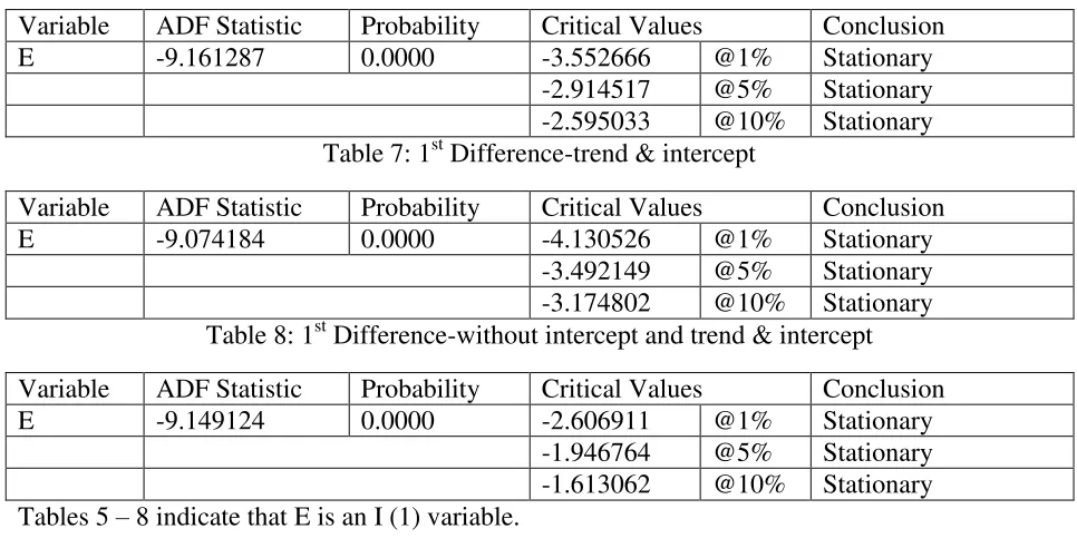
[image:7.612.172.440.398.661.2]Stability Test of the ARIMA (0, 1, 1) Model
Figure 2
-1.5 -1.0 -0.5 0.0 0.5 1.0 1.5
-1.5 -1.0 -0.5 0.0 0.5 1.0 1.5
M
A
r
o
o
ts
Since the corresponding inverse roots of the characteristic polynomial lie in the unit circle, it illustrates that the chosen ARIMA (0, 1, 1) model is stable and suitable for predicting inflation in Egypt over the period under study.
FINDINGS
Descriptive Statistics
Table 13
Description Statistic
Mean 9.6914
Median 9.95
Minimum -3
Maximum 29.5
Standard deviation 6.8439
Skewness 0.46478
Excess kurtosis -0.063052
As shown above, the mean is positive, i.e. 9.6914%. The minimum is -3% and the maximum is 29.5%. The skewness is 0.46478 and the most striking characteristic is that it is positive, indicating that the inflation series is positively skewed and non-symmetric. Excess kurtosis was found to be -0.063052; implying that the inflation series is not normally distributed.
Results Presentation1
Table 14
ARIMA (0, 1, 1) Model:
∆𝐸𝑡−1= −0.364872𝜇𝑡−1… … … . . … . [3]
P: (0.0107) S. E: (0.1429)
Variable Coefficient Standard Error z p-value
MA (1) -0.364872 0.142939 -2.553 0.0107**
Predicted Annual Inflation in Egypt
Table 15
Year Prediction Std. Error 95% Confidence Interval
2018 23.3 4.90 13.7 - 32.9
2019 23.3 5.81 11.9 - 34.7
2020 23.3 6.59 10.4 - 36.2
1
2021 23.3 7.29 9.0 - 37.6
2022 23.3 7.93 7.7 - 38.8
2023 23.3 8.52 6.6 - 40.0
2024 23.3 9.07 5.5 - 41.1
2025 23.3 9.59 4.5 - 42.1
2026 23.3 10.08 3.5 - 43.0
2027 23.3 10.55 2.6 - 44.0
After the Egyptian pound’s floatation in November 2016, the Central Bank of Egypt (CBE) drastically tightened its monetary policy (BNP PARIBAS, 2018) and this move is also justified by Table 15 above; which clearly shows that inflation in Egypt is projected to be hovering around 23.3% in the next 10 years. This could be attributed to import prices as well as the energy subsidy reform that was recently implemented in Egypt. It is also important to note that monetary factors such as an increase in portfolio investment inflows and the return of foreign currency liquidity into the banking system also played a pivotal role in inflating the economy. This is very bad for the Egyptian economy and the urgent need to control inflation cannot be ruled out.
CONCLUSION
The ARIMA model was employed to investigate annual inflation rates in Egypt from 1960 to 2017. The study planned to forecast inflation in Egypt for the upcoming period from 2018 to 2027 and the best fitting model was carefully selected based on the minimum AIC value. The ARIMA (0, 1, 1) model is stable and most suitable model to forecast inflation in Egypt for the next ten years. Based on the results, policy makers in Egypt should continue to engage proper economic policies in order to fight against persistent inflationary pressures in the economy. In this regard, the CBE is encouraged to continue tightening up its monetary policy in line with its inflation-targeting regime in order to restore macroeconomic stability in the country.
REFERENCES
[1] Blanchard, O (2000). Macroeconomics, 2nd Edition, Prentice Hall, New York.
[2] BNP PARIBAS (2018). Egypt – Gradual monetary easing, PNP PARIBUS.
[3] Box, G. E. P & Jenkins, G. M (1976). Time Series Analysis: Forecasting and Control, Holden Day, San Francisco.
[4] Brocwell, P. J & Davis, R. A (2002). Introduction to Time Series and Forecasting, Springer, New York.
[6] Chatfield, C (2004). The Analysis of Time Series: An Introduction, 6th Edition, Chapman & Hall, New York.
[7] Cryer, J. D & Chan, K. S (2008). Time Series Analysis with Application in R, Springer, New York.
[8] Enke, D & Mehdiyev, N (2014). A Hybrid Neuro-Fuzzy Model to Forecast Inflation, Procedia Computer Science, 36 (2014): 254 – 260.
[9] Hector, A & Valle, S (2002). Inflation forecasts with ARIMA and Vector Autoregressive models in Guatemala, Economic Research Department, Banco de Guatemala.
[10] Hosny, A. S (2016). What is the Central Bank of Egypt’s implicit inflation target? International Journal of Applied Economics, 13 (1): 43 – 56.
[11] King, M (2005). Monetary Policy: Practice Ahead of Theory, Bank of England.
[12] Moriyama, K (2011). Inflation inertia in Egypt and its policy implications, Middle East and Central Asia Department, IMF.
[13] Nyoni, T & Nathaniel, S. P (2019). Modeling Rates of Inflation in Nigeria: An Application of ARMA, ARIMA and GARCH models, Munich University Library – Munich Personal RePEc Archive (MPRA), Paper No. 91351.
[14] Nyoni, T (2018). Modeling and Forecasting Inflation in Kenya: Recent Insights from ARIMA and GARCH analysis, Dimorian Review, 5 (6): 16 – 40.
[15] Nyoni, T (2018). Modeling and Forecasting Inflation in Zimbabwe: a Generalized Autoregressive Conditionally Heteroskedastic (GARCH) approach, Munich University Library – Munich Personal RePEc Archive (MPRA), Paper No. 88132.
[16] Nyoni, T (2018). Modeling Forecasting Naira / USD Exchange Rate in Nigeria: a Box – Jenkins ARIMA approach, University of Munich Library – Munich Personal RePEc Archive (MPRA), Paper No. 88622.
[17] Nyoni, T. (2018). Box – Jenkins ARIMA Approach to Predicting net FDI inflows in Zimbabwe, Munich University Library – Munich Personal RePEc Archive (MPRA), Paper No. 87737.
[18] Wei, W. S (2006). Time Series Analysis: Univariate and Multivariate Methods, 2nd Edition, Pearson Education Inc, Canada.