Original citation:
Rock, Kat, Brand, Samuel, Moir, Jo and Keeling, Matthew James. (2014) Dynamics of infectious diseases. Reports on Progress in Physics, Volume 77 (Number 2). Article number 026602.
Permanent WRAP url:
http://wrap.warwick.ac.uk/61984
Copyright and reuse:
The Warwick Research Archive Portal (WRAP) makes this work of researchers of the University of Warwick available open access under the following conditions. Copyright © and all moral rights to the version of the paper presented here belong to the individual author(s) and/or other copyright owners. To the extent reasonable and practicable the material made available in WRAP has been checked for eligibility before being made available.
Copies of full items can be used for personal research or study, educational, or not-for-profit purposes without prior permission or charge. Provided that the authors, title and full bibliographic details are credited, a hyperlink and/or URL is given for the original metadata page and the content is not changed in any way.
Publishers statement:
http://dx.doi.org/10.1088/0034-4885/77/2/026602 A note on versions:
The version presented here may differ from the published version or, version of record, if you wish to cite this item you are advised to consult the publisher’s version. Please see the ‘permanent WRAP url’ above for details on accessing the published version and note that access may require a subscription.
Dynamics of Infectious Diseases
Kat Rock1,2 Sam Brand1,2 Jo Moir1,2 Matt J. Keeling1,2,3†
1
- WIDER Centre, University of Warwick
2
- Mathematics Institute, University of Warwick
3 - School of Life Sciences, University of Warwick
†−
To whom correspondence should be addressed, [email protected]
Abstract
Modern infectious disease epidemiology has a strong history of using mathe-matics both for prediction and to gain a deeper understanding. However the study of infectious diseases is a highly interdisciplinary subject requiring insights from multiple disciplines, in particular a biological knowledge of the pathogen, a statisti-cal description of the available data and a mathematistatisti-cal framework for prediction. Here we begin with the basic building blocks of infectious disease epidemiology – the SIS and SIR type models – before considering the progress that has been made over the recent decades and the challenges that lie ahead. Throughout we focus on the understanding that can be developed from relatively simple models, although accurate prediction will inevitably require far greater complexity beyond the scope of this review. In particular, we focus on three critical aspects of infectious disease models that we feel fundamentally shape their dynamics: heterogeneously struc-tured populations; stochasticity; and spatial structure. Throughout we relate the mathematical models and their results to a variety of real-world problems.
1
Introduction
Infectious diseases pose a considerable challenge to modern life. In the 1950s and 60s, with the development of safe vaccines and antibiotics it was largely felt that this age-old foe was beaten. However, recent experience with the evolution of drug-resistant pathogens, the emergence of new infections and the challenges of cost-effective control highlight that we are still a long way from eradicating most diseases. This review is fo-cussed upon how tools from mathematics and theoretical physics can provide meaningful insights into infectious disease dynamics and hence provide both a general understand-ing of the patterns and processes as well as enable a thorough understandunderstand-ing of the impact of proposed control measures.
(termed phage), while higher organisms often have a range of specific pathogens that depend on these organisms for their survival. Examples of high impact and high profile infections exist from every group of living organisms: agricultural crops are commonly infected with fungal or viral pathogens [223]; wild plant populations can be devastated by infection (such as Sudden Oak Death [94]); insects also suffer with honey bees being a notable example potentially related to Colony collapse disorder [86]; amphibians are likewise infected, with Chytrid fungus destroying populations of frogs worldwide [61]. However, infection in mammals has received by far the most attention both due to the impact on livestock production systems (eg Foot-and-Mouth disease [147, 90] or Clas-sical Swine Fever [137]) and the effects on human health. Globally, it is estimated that one quarter of all human deaths are due to infectious diseases [254].
This review focuses on infectious diseases, those illnesses caused by an infecting organism that can be spread between individuals. This broad definition includes well-known viral infectious such as measles, influenza and HIV or bacterial infections such as meningitis and cholera, but also includes infection with fungal pathogens, proto-zoa (such as the organism that causes malaria) and larger parasites (such a helminths and other worms). Throughout this review, we generally focus on viral or bacterial pathogens, as these are most commonly studied in the literature, and we will generally use the term pathogen to refer to any infecting organism.
understand-ing of infectious disease dynamics before describunderstand-ing the complexities that would need to be included to make such models practically useful.
The epidemiology of infectious diseases is a complex and multi-factoral subject [16, 151, 74]. As such, no single review can hope to cover all aspects. Here we fo-cus largely on the population dynamics of infectious diseases – how the number of individuals infected changes dynamically over time. This article therefore relies heavily on tools from mathematics and theoretical physics (the theory of differential equations and dynamical systems, statistical mechanics, and stochastic processes). However, there are multiple disciplines that feed into epidemiology that we do not cover. Statistics is one with which many readers will be familiar; statistics plays a vital role in both inter-preting the observed infection data (accounting for the many biases in reporting) and in parameter inference when we attempt to fit models to data. Obviously, a range of biological sciences from microbiology to immunology to ecology are needed to inform our understanding of the pathogen, the host and their interaction; while we do not attempt a comprehensive review of such knowledge, the next section does provide suf-ficient biological background to motivate and justify the choice of model formulation. Finally, in recent years it has become apparent that other disciplines have a role to play: economics is vital to underpin cost-effectiveness studies that are key to assessing control programmes; sociology and psychology help to explain and predict human response to outbreaks or new treatments; while medical insights are needed to understand the link between the individual as a host for the pathogen and the individual as a patient that requires treatment. Therefore, when developing models for the spread of an infectious disease we not only need a range of mathematical skills but must account for the in-sights provided by many other disciplines. Throughout, we had attempted to draw on citations from the mathematical and biological literature whenever possible, so as to introduce the reader to this (possible novel) fields of scientific publication.
2
Basic Models
With only a very few exceptions, most mathematical descriptions of the population dy-namics of infectious diseases rely on being able to partition the population into discrete non-overlapping compartments [15, 180, 16, 151, 74]. This act of compartmentalisation allows us to study the dynamics of infection by capturing the transition of individuals between compartments. A simple example will illustrate the main points (Figure 1): before the 2009 H1N1 (swine-flu) pandemic very few people in the population had seen a similar infection before and could therefore be categorised as Susceptible, suscepti-ble people that come in contact with the pathogen can become Infected and pass the pathogen (influenza virus) on to other susceptible individuals, after a time infected peo-ple generally ‘fight-off’ the infection, are no-longer able to transmit and are classified asRecovered. This simply natural history of infection is familiar to us all, and the com-partmentalisation into the three categories Susceptible, Infected and Recovered allows us to develop simple mathematical models. Throughout the early sections of this re-view, we will illustrate such compartmental models using the caricature method shown in Figure 1. However, before we write these models in terms of differential equations, there are two fundamental points that need emphasis.
S I R
infection
Figure 1: Compartmental caricature of the basic SIR model (solid lines show transition or movement between classes; dashed lines show the action of transmission)
Firstly, in the description above we have taken a pathogen-centric view, categorising the host (person) by their status with respect to the pathogen – this is an epidemio-logical view-point and is necessary if we wish to study the pathogen dynamics. More commonly we are accustomed to a medical perspective where we think about the status of the patient and what symptoms they display. Sometimes these two view-points are aligned and severe illness coincides with the peak of infectivity, however many other scenarios are plausible; for example, with chickenpox (caused by the varicella zoster virus) the peak of infection generally occurs a few days before the onset of a rash and other symptoms [151].
multiple times; sexually transmitted infections (STIs) tend to follow this profile and in-dividuals that are treated for infection generally return to the susceptible class, giving rise to SIS (Susceptible, Infected, Susceptible) models. It is na¨ıve to think that the amount of pathogen an individual can transmit is constant throughout the time that they are infected, clearly following infection (with a low level of the infecting pathogen) there needs some time for the pathogen to build to sufficient levels for onward trans-mission to be likely. This effect can be captured by adding an additional Latent (or Exposed) class that individuals need to pass through before they become infectious (ie actively transmitting).
Finally, we stress that although we begin this exploration of infectious disease dy-namics by considering simple systems of ordinary differential equations (ODEs), their formulation may be motivated by considering the stochastic behaviour of individuals. In particular, following the work of [167] we can consider the ODEs as the limit of a stochastic process where a large (infinite) number of individuals are moving between the various model compartments. In this limit of infinitely many individuals, the stochastic movement between compartments can be conceptualised as a continuous flow. Section 4 provides more details of this stochastic approach and the connections to the deter-ministic models of sections 2 and 3.
2.1 A Generic Model
We can now put these elements together to create a generalised model for the dynamics of infection in a population [15, 180, 16] (see Figure 2):
Susceptibles dSdt = B + νR − λS − dS
Exposed dEdt = λS − αE − dE
Infectious dIdt = αE − γI − dI
Recovered dRdt = γI − νR − dR
(1)
Equation (1) contains one rate (B) which determines the rate at which new-born indi-viduals enter the population, and five per capita rates (ν,d,α,γ andλ) that determine transitions between (or out of) categories. In this form the dynamics could be solved relatively trivially, however there is an additional non-linear feed-back that needs to be incorporated. TheForce of Infection (λ) which quantifies the risk of infection is clearly related to the number of infectious individuals in the population. In particular it is standard to assume:
Force of Infection λ = βI/N (2)
force of infection becomes modified in spatial models where we account for non-random mixing. In Equation (2) we have assumed Frequency dependent transmission; this is derived by assuming that each individual has a fixed number of daily contacts that is independent of population size, hence the force of infection is related to the frequency of infectious individuals in the population. Frequency dependent transmission tends to be the norm for human populations. The alternative is to assume Density dependent transmission where more dense populations give rise to more contacts and hence the force of infection is related to the density of infectious individuals: λ=βI. However, in many theoretical settings it is often simpler to re-scale the variables such that the pop-ulation size, N, is one; although clearly this is not feasible when dealing with changing population sizes. Under such a re-scaling the two transmission assumptions are equiv-alent.
S λ E α I γ R
infection
ν B
d d d d
Figure 2: Compartmental caricature of the generic SEIRS model (solid lines show tran-sition or movement between classes; dashed lines show the action of transmission; arrows entering or leaving the system correspond to births and deaths respectively).
Together Equations (1) and (2) combine to generate a range of infection models that can either be studied analytically or be rapidly integrated numerically. We first highlight the three standard models that are contained within this more general for-mulation. The simple SIR model is recaptured by setting B = d= ν = 0 and letting
2.2 Early Behaviour
One of the most fundamental concepts in epidemiology is theBasic Reproductive Ratio
or Number, represented by R0. This quantity is defined as “The average number of
secondary cases produced by an average infected individual in a totally susceptible population”, and in practice provides a quantitative guide to both invasion and control of an infectious disease [15, 180, 16, 123]. In particular, whenR0 is greater than one an infection invading a na¨ıve population can spread whereas whenR0is less than one chains of infection will always die out. These logical arguments can be made mathematically precise by calculating the Jacobian of the disease free equilibrium (S = N, E = I =
R= 0). For the general model defined by equations (1) and (2), the Basic Reproductive Ratio can be calculated in three parts considering the dynamics associated with a newly infected individual: the probability a newly infected individuals goes on to become infectious; the rate at which new cases are then generated; and the average duration over which the individual remains infectious.
R0 =
α
α+d × β S N ×
1
γ+d
= βα
(α+d)(γ+d) ≈
β
γ . (3)
Equation (3) has been gained by noting that it is calculated when everyone is susceptible (S =N) while the approximation holds if the natural death-rate is small compared to the rates of transition through the exposed and infectious classes. Two points are imme-diately noteworthy in the calculation ofR0. The first is that many of the components of the full SEIRS model do not play a role in the value ofR0, in particular it is independent of both the birth rate and whether (or not) there is waning immunity; thus the SIR and SIS models have the same basic reproductive ratio for the same parameters despite the differences in underlying structure. Secondly, the value ofR0 depends on the trans-mission rateβ, which in turn depends on the rate at which (epidemiologically-relevant) contacts are made. We therefore find that R0 depends on both the pathogen and the population. For example although measles and influenza are both spread through close-contact or local airborne interactions,R0 for measles is around 17 [16] whereasR0 for influenza is between 1.5 and 3.0 [239]. Considering HIV infection illustrates the role of the contacts, with values of R0 during the 1980s estimated as in the range 2-5 in the UK, but 10-12 in sub-Saharan Africa [16].
0 500 1000 1500 2000 2500
10−6
10−5
10−4
10−3
10−2
10−1
100
Time (days)
Proportion of Population Infectious, I
SIS model
SIR model
[image:9.612.165.445.231.454.2]SEIRS model
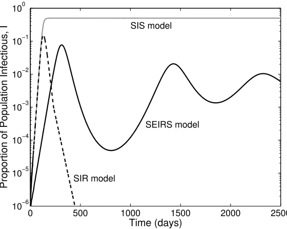
Figure 3: Comparison of the basic infection models derived from equations (78) and (2). The three curves show the proportion of infectious individuals in the population (I/N), for the standard SIS model, the standard SIR model and the general SEIRS model. (For all three models: β = 0.2, γ = 0.1. For the SIS model B = d = 0 and
α = ν → ∞; for the SIR model B = d = ν = 0 and α → ∞; for the SEIRS model
B =d= 10−4,α = 0.1 andν = 10−3. All rates are given in days−1 (I(0) =I0 = 10−6,
be more closely linked to available data. From consideration of the disease-free state of the general model, the early growth rate is given by:
r = 1 2
hp
4S0βα+ (α−γ)2−(α+γ+ 2d)
i
(4)
rSIR = rSIS = S0β−γ−d
whereS0(=S(0)/N) is the proportion of the population susceptible at the start of the outbreak. This raises an interesting and important applied issue, when we observe an exponential growth of cases in the early phase of an epidemic; there are currently no ro-bust techniques for distinguishing between a small scale epidemic where all cases report symptoms of infection and a large scale epidemic where only a small proportion report [18]. In general it is not until the epidemic peaks and we observe strong non-linear effects that this distinction can be made.
2.3 Long-term Behaviour
Examining Figure 3 also leads us to think about the long-term dynamics of this system. We first begin by considering a general solution before focussing on the specific cases of the SIS and SIR models. When considering long-term endemic behaviour, it is customary to set B = d which effectively rescales the population size N = 1. Under this assumption the equilibrium dynamics are given by:
S∗ = (α+dβα)(γ+d) ≈ γ
β E∗ = (βα−(α+d)(γ+d))(ν+d)(γ+d)
βα(αν+νγ+αγ+αd+νd+γd+d2) ≈
(β−γ)(ν+d)γ β(αν+νγ+αγ)
I∗ = (βα−(α+d)(γ+d))(ν+d)
β(αν+νγ+αγ+αd+νd+γd+d2) ≈
α(β−γ)(ν+d)
β(αν+νγ+αγ)
(5)
where again the approximations hold whenever the natural death-rate is small compared to the rates of transition through the exposed and infectious classes. In general this equilibrium is approached through a series of damped oscillations, which may interact with any seasonal forcing in the basic parameters [153]. It should be noted that the susceptible equilibrium is only viable (i.e. S∗ ≤ N = 1) when the basic reproductive ratio is greater than one; when the basic reproductive ratio is less than one only the disease free equilibrium is a viable fixed point of the system. It is worth noting that at the equilibrium we have that (S∗ = 1/R0), this is a common feature of many epi-demiological models and it related to the fact that at equilibrium the average number of secondary cases produced per infected individual (Re =R0×S/N) has to be equal to one, otherwise the number of case would change.e.
For the SIS model, the dynamics simplify enormously. In particular we now have the equilibrium solution:
SSIS∗ = γ
β I
∗
For this model, the recovery of infected individuals back to the susceptible state is sufficient to maintain the presence of infection, and the fact that there are only two compartments means thatS+I = 1. In fact, the SIS model is equivalent to the logistic growth model in ecology, and therefore has an algebraic solution:
ISIS(t) = (β−γ)I0e (β−γ)t
(β−γ) +I0β
h
e(β−γ)t−1
i
whereI0 is the proportion of infection in the population att= 0.
In contrast, the simple SIR model without births and deaths does not have an en-demic equilibrium; instead there is a single epien-demic which eventually dies out. This extinction of infection is caused by a depletion of susceptibles to a level that cannot sustain the infection, without new births or waning immunity there is no way for the susceptibles to be replenished and so the infection is doomed to extinction. Mathe-matically, this is clear from the fact that the disease-free states are the only equilibria. However, for the simple SIR the key question is how many individuals become infected during the entire course of the epidemic, this addresses an issue of fundamental concern for any outbreak – how big is the epidemic likely to be. The solution to this problem dates back to the ground-breaking papers of Kermack and McKendrick [155], and arises from considering dRdS = dSdt/dRdt. The Final Epidemic Size,R∞ is given by the relation:
R∞=S0[1−exp(−R0R∞)] (6)
whereR0 is the basic reproductive ratio, S0 is the initial proportion of the population that is susceptible to infection and R∞ is the proportion of the population that have passed through the infectious class (specifically R∞ =S(0)−S(∞) assuming a small initial seed of infection). We find that an identical formula holds for SEIR-type models, all that is important is the lack of births, deaths and waning immunity. What is clear from this formula is that there will always be some individuals that escape an epidemic, although the proportion of the population that do escape becomes small asR0 becomes large. We note that in practice epidemics rarely infect very high proportions of the population and this is largely due to heterogeneities in risk (see below) with some in-dividuals with high risk contributing most to the value of R0 whereas others with low risk more likely to escape infection. Hence, the final epidemic size should be viewed as an idealized calculation, although for the recent H1N1 (swine-flu) outbreak the value of
R∞≈0.37 (derived from R0 ≈1.25 [18]) is in good qualitative agreement with finding from detailed serological studies [56].
2.4 Greater realism, more compartments
realism can be introduced by including more compartments and therefore greater het-erogeneity in the dynamics. Later we discuss multiple compartments based on the host, allowing us to consider age-structured models or multiple host species. Here we focus on additional compartments due to the pathogen. Two approaches are worth highlighting in detail.
One way in which additional compartments may be required is when there is a more complex natural history of infection that needs to be captured. For example, we may wish to have a short-duration Maternal Immunity class that individuals are born into, individuals in this class would be protected against infection due to immunity gained from the mother. Alternative, there are infections (such as typhoid) where carrier indi-viduals exist who may be weakly infectious for extremely long periods of time or who may intermittently revert to a highly infectious state; in such cases these additional compartments need to be included in any model to produce realistic results. However, the inclusion of these extra compartments is not conceptually challenging and uses the existing framework that specifies the rates of entering and leaving each compartment, although parameterisation of such models may be much more complex.
An additional way in which more compartments can be included is to subdivide the infectious (and exposed) classes into more groups. Ignoring waning immunity this would lead to the following set of equations:
Susceptibles dSdt = B − λS − dS
Exposed dE1
dt = λS − α1E1 − dE1
Exposed dEndt = αn−1En−1 − αnEn − dEn n= 2, . . . , m
Infectious dI1
dt = αmEm − γ1I1 − dI1
Infectious dIndt = γn−1In−1 − γnIn − dIn n= 2, . . . , M
Recovered dRdt = γMIM − dR
Force of Infection λ = P
nβnIn/N
(7)
S E1 Em
I1
IM R
λ α1 αm−1
αm
γ1
γM−1
γM B
d d d
d d
d
[image:13.612.141.474.94.301.2]infection
Figure 4: Compartmental caricature of the multi-compartmental SE1. . .EmI1. . .IMR
model (solid lines show transition or movement between classes; dashed lines show the action of transmission; arrows entering or leaving the system correspond to births and deaths respectively).
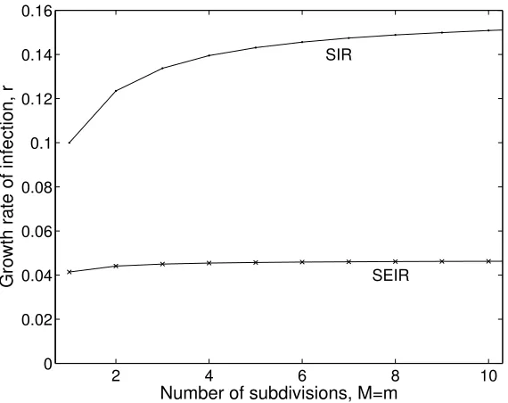
number of secondary cases produced by infected individuals, which in turn influences persistence [152, 174, 63]. In contrast, by having multiple exposed and infectious classes that an individual must transition through before recovery, the total time spent in all these classes is given by a gamma distribution. These multiple classes both act to speed the growth rate of infection in the population (see Figure 2) and lead to less variability in individual behaviour. In practice there is rarely sufficient data to necessitate more than two or three exposed and infectious classes (m = M = 3). The individual-level implications of this additional structure is considered in more detail in Section 4.4.2.
Here we have stressed the need to include multiple compartments (that reflect the underlying biology) in any attempt to generate reliable predictions. However, writing down such models in inherently unwieldy, and while necessary for accurate prediction it adds comparatively little to our deeper understanding of the dynamics. Therefore, in the sections that follow we often focus on how different elements (risk-structure, stochasticity or spatial structure) effect the simple SIR and SIS models, and we leave it to the reader to extrapolate in the obvious manner for models with more compartments.
2.5 Vaccination
2 4 6 8 10 0
0.02 0.04 0.06 0.08 0.1 0.12 0.14 0.16
SIR
SEIR
Number of subdivisions, M=m
[image:14.612.165.450.229.455.2]Growth rate of infection, r
whereas only a proportion of these will be immunised and protected against infection. With the best vaccines the proportion that are protected can be very high, often in excess of 99%, however with other vaccines, such as those against seasonal influenza where the vaccine is developed based on predictions of future strains, the effectiveness can be anywhere between 30 and 90% [38]. In the remainder of this section we therefore formulate models based on the level (rate or proportion of the population) of successful immunisation, with the implicit assumption that this would necessitate a higher level of vaccination.
Vaccination is generally more common in diseases that naturally obey the S(E)IR-type paradigm (rather than SIS-S(E)IR-type infections). This is because vaccines generally operate by triggering the host’s own natural immunity to the infecting pathogen, with-out causing disease. A suitable equation for the dynamics of an SIR-type infection with vaccination would be:
Susceptibles dSdt = B(1−p) − λS − dS − vS/N
Infectious dIdt = λS − γI − dI
Recovered dRdt = γI − dR
Vaccinated dVdt = Bp + vS/N − dV
Force of Infection λ = βI/N.
(8)
Here vaccination takes two forms (although generally either one or the other domi-nates); firstly a proportion p of new-borne individuals are vaccinated and successfully immunized and so enter the compartment V where they remain for life. Secondly we assume a random vaccination (and immunization) rate v, and if the randomly selected individual is susceptible then they are transfered to the V compartment. The first of these is most common and equates to the typical childhood immunization campaigns that have been so successful in reducing childhood mortality; the second of these is associated with vaccinating to control a novel outbreak (such as influenza pandemic [18] or foot-and-mouth [236]), or vaccinating wild animal populations [253, 7, 57]. It should be noted that p refers to the proportion of new-borns immunised and therefore lies between 0 and 1, whereasv is a rate and therefore is only constrained by resources and logistics.
We first focus on the use of vaccination to eradicate infection. This can be ap-proached in two ways: the first is to consider if (long-term) vaccination can prevent an infection invading and spreading from the disease-free equilibrium; the second is to consider the equilibrium state and how the prevalence of infection changes with vacci-nation. Looking at the disease-free equilibrium with vaccination (and assumingB =d
and henceN = 1) we find:
S∗ = 1−p
1 +v/d V
∗
= 1− 1−p
S I R
V
λ γ1
B(1−p)
v/N
Bp
d d d
d
Figure 6: Compartmental caricature of the SIRV model (solid lines show transition or movement between classes; dashed lines show the action of transmission; arrows entering or leaving the system correspond to births and deaths respectively).
Examining the early growth rate of infection from this point gives:
dI
dt = (βS ∗−
γ−d)I
and hence the disease fails to invade (has negative growth rate) if
S∗ < γ+d
β =
1
R0
.
Therefore, we require immunity due to vaccination to be sufficient to drop the proportion of susceptibles in the population below their non-vaccinated equilibrium value in the presence of infection. What is important to realise is that it is not necessary to immunise everyone to protect the entire population, the action of immunising one person has additional benefits to other individuals who could have been infected by this person. This level of addition protection in the population is known asherd-immunity[16, 151, 74]. Therefore vaccination is an altruistic act which benefits both the individual and the population. Examining the two methods of vaccination separately gives critical thresholds:
pc = 1− 1
R0
vc = (R0−1)d (9)
Immunising above these thresholds prevents a pathogen from successfully invading.
Alternatively, we can consider the equilibrium state with both infection and vaccina-tion acting to reduce the susceptible populavaccina-tion, again assumingB =d. Two equilibria are possible depending upon whether the level of vaccination is sufficient to eradicate infection or not:
S∗ = R1 0
I∗ = d(R0−1)β−pdR0−v or
S∗ = 1−p 1 +v/d I∗ = 0
−1000 −50 0 50 100 150 200 0.5
1 1.5 2 2.5 3 3.5 4 4.5 5
x 10−4
Time (years)
[image:17.612.164.446.101.333.2]Prevalence of Infection, I
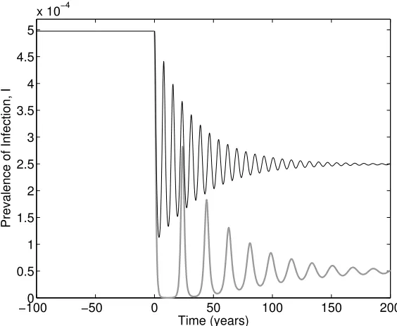
Figure 7: Illustration of the honeymoon effect for vaccination in the standard SIR model and two levels of vaccination. Vaccination begins at time 0, when the system is at its unvaccinated equilibrium. Two levels of vaccination at birth are considered p = 0.25 (black line) and p = 0.45 (thick grey line), noting that the critical threshold occurs at pc ≈ 0.5. (The SIR model is given by: β = 0.2, γ = 0.1, α → ∞, ν = 0 and
B =d= 10−4; with all rates being in days−1).
Hence we find that immunisation has a linear impact on the prevalence of infection; the proportion of infected individuals drops linearly with both types of vaccination until it reaches zero at the critical thresholds. This is an important public-health observation, as it generally means that it is better to do some vaccination even if there is not suffi-cient resources (or demand) to reach the critical threshold. The exceptions to this rule are when there exists complex interactions between disease severity and age-structure [8] as vaccination generally increases the average age of infection (see Section 3.2).
honeymoon effect [184]– before rising to much higher levels (when concerns about the vaccine programme are likely to be raised). Figure 7 illustrates this behaviour for two levels of vaccination given at birth below the critical threshold; not only do we observe large oscillations and substantial honeymoon effects, but also we note how long it can take for the dynamics to approach equilibrium. Given that this form of vaccination only occurs at birth the time-scales of the programme are comparable with the time-scales of the host life-cycle; this is why new vaccinate campaigns are often accompanied by catch-up programmes in older age-groups.
Again, there are multiple improvements that can be made to the standard model of vaccination (Equation 8). Clearly, adding an exposed class and subdividing the exposed and infectious classes into sub-compartments will increase the realism of the infection dynamics (although this will have limited impact on the critical eradication thresholds). When waning immunity is a feature of the infection dynamics (ν >0) then it becomes natural to also include this facet in the vaccination dynamics, with the possibility of a different rate of waning immunity to capture the fact that protection following infection may be more long-lasting than that due to vaccination. In addition, for many vaccines a single dose is insufficient to provide life-long immunity and therefore the impact of booster vaccines later in life must be incorporated into the standard equations [4]. How-ever, two improvements are particularly interesting from a practical perspective: those concerning the use of vaccines in controlling novel outbreaks, and those that consider in more detail the action of the vaccine itself.
Vaccination is often seen as a panacea against infection, and for many endemic diseases where there is a childhood vaccination campaign this is generally the case. However, vaccination can also be used reactively in the face of an on-going outbreak. Classic examples include the use of vaccination to control bioterrorist use of small-pox [92, 130] or pandemic influenza [88] in humans, or to limit the spread of livestock infections such as foot-and-mouth disease [236]. In these reactive situations two modi-fications are important. Firstly, there is generally a delay (of between a few days and several weeks) between receiving the vaccine and being protected, which in turn de-lays the impact of vaccination. Mathematically this can be captured by sub-dividing the vaccinated compartment into P classes and allowing susceptibility to infection to decrease as an individual moves through the classes; therefore immediately following vaccination protection in limited and it is possible to acquire the infection. Secondly, the assumption of random vaccination can be refined, only vaccinating individuals that have not yet received the vaccine. The new equations become:
Susceptibles dSdt = B − λS − dS − vS/(S+I +R)
Infectious dIdt = λS + P
nσnλVn − γI − dI
Recovered dRdt = γI − dR
Vaccinated dV1
dt = vS/(S+I+R) − µ1V1 − σ1λV1 − dV1
Vaccinated dVndt = µn−1Vn−1 − µnVn − σnλVn − dVn
Vaccinated dVPdt = µP−1VP−1 − σPλVP − dVn
Here the delay from vaccination to immunity weakens the impact of this control, whereas the refinement in the vaccination procedure increases the speed at which herd-immunity can be reached.
S I R
V1
Vn
λ γ1
B
v/N
d
d
d d d
µ1
µn−1
σ1λ
[image:19.612.181.434.158.408.2]σnλ
Figure 8: Compartmental caricature of the SIRV model (solid lines show transition or movement between classes; dashed lines show the action of transmission; arrows entering or leaving the system correspond to births and deaths respectively).
using this leaky vaccine concept.
Susceptibles dSdt = B(1−p) − λS − dS
Infectious dIdt = λS − γI − dI
Recovered dRdt = γI − dR
Vaccinated, uninfected dVdt = Bp − λσV − dV
Vaccinated, infectious dJdt = λσV − γρJ − dJ
Force of Infection λ = βI/N + βτ J/N.
(12)
where the effect on vaccination on susceptibility, transmission and recovery are captured by the parameters σ(≤ 1), τ(≤ 1) and ρ(≥ 1). By considering the invasion of the disease-free equilibrium we can again derive the critical eradication threshold:
pc =
R0−1
R0−RV
RV = τ σβ ργ+d
whereRV is the equivalent of the basic reproductive ratio when the entire population is
vaccinated. From this formulation it is clear that any of these three actions (separately or in combination) can lead to eradication of the infection as long asRV <1.
S I R
V J
λ γ
B(1−p)
Bp
d d d
d d
λσ
Figure 9: Compartmental caricature of the generic SIRVJ model (solid lines show transi-tion or movement between classes; dashed lines show the actransi-tion of transmission; arrows entering or leaving the system correspond to births and deaths respectively).
3
Heterogeneous Populations
which affect the spread or transmission of disease. Sometimes it may be easy to com-partmentalise a population, not only according to disease status (e.g. S,E,I,R), but also by another natural partition of the population; for multiple species this is particularly easy, as each different species would form its own category. Conversely it may be hard to decide upon exactlyhowit is best to separate out a varying range of behaviour; for instance for STIs (sexually transmitted infections), where the number of sexual partners an individual has puts them at differential risks of contracting a disease, it is far from obvious how to determine where the boundary between “low risk” and “high risk” lies. Similarly when dealing with age-structure, it is unclear how to partition the population into discrete age-classes.
In the SIR modelling framework, instead of having just three states (according to infection status) there are now three states per population category. In the case of two populations (these can be thought of as two different species in this example) the SIR diagram (without demography) now looks a little different (see Figure 10).
S1 I1 R1
S2 I2 R2
β12
β21
β22
[image:21.612.170.443.318.481.2]β11
Figure 10: Compartmental caricature of the basic two-population SIR model.
In the standard SIR model transmission of the pathogen between all individuals in the population is assumed to be governed by a single rate parameters (β) which is equivalence to assuming that all individuals mix randomly with each other. When the population is heterogeneous, we have the opportunity to allow different transmission rates within and between the classes. In particular, the transmission terms now depend upon who acquires infection from whom, and these new rates are now give by terms of the form βTo From (i.e. β21 denotes the transmission rate of disease going to species 2 from species 1).
as a weighted sum. For speciesithe SIRdynamics are given by,
Susceptibles dSidt = Bi − λiSi − diSi
Infectious dIidt = λiSi − γiIi − diIi
Recovered dRidt = γiIi − diRi
Force of Infection λi = PjβijIj
(13)
This transmission interdependence becomes more obvious if we write in full a two-class model and SIR dynamics :
Susceptibles dS1
dt = −β11S1I1−β12S1I2
Class 1 Infectious dI1
dt = β11S1I1+β12S1I2−γI1
Recovered dR1
dt = γI1
Susceptibles dS2
dt = −β21S2I1−β22S2I2
Class 2 Infectious dI2
dt = β21S2I1+β22S2I2−γI2
Recovered dR2
dt = γI2
(14)
where the force of infection for each classλihas been included explicitly, and we have
scaled the population size to one. This formulation for transmission can be represented more succinctly in the form of a transmission matrix known as the WAIFW (or Who Acquires Infection From Whom) matrix:
β=
β11 β12
β21 β22
(15)
This allows the change of infectious individuals to be written in vector notation:
dI
dt =S.βI−γI (16)
The same heterogeneous population structure, transmission matrix and vectorisation concepts can be applied in a similar fashion to SEIR, SIS and other models of disease progression.
In the unstructured SIR model (see Section 2) parameterisation of the infection rate,
β, is relatively easy and is often derived from the equilibrium dynamics; in particular given thatS∗ =γ/β and both the proportion seronegative (susceptible) and the dura-tion of infecdura-tion can be measured with relative ease, calculating β is not conceptually challenging. However, in heterogeneous populations where we have partitioned the host intonclasses, estimating the matrix, βin much harder as there are nown2 entries and often data for just n different data points. This means that often we are only able to estimate n parameters within the WAIFW matrix, and in general any matrix with n
this is done depends on the specific population, the disease being modelled and the epidemiological understanding of the transmission routes [110]. This will be discussed in more detail below.
3.1 Heterogeneous Reproductive Ratio
As for single homogeneous population models, being able to estimate the basic repro-ductive ratio,R0, for heterogenous populations is highly desirable. As before this ratio may be derived from first principles by considering how individuals become infected and generate secondary cases. We will begin with a two-population model, although the argument generalises to multiple populations. The basic reproductive ratio for an infected individual in population 1 or 2 (R01 and R02 respectively) can be found as in Section 2.2:
R01 = Average infectious period of 1s×
(rate of generating infected 1s + rate of generating infected 2s)
= 1
γ1
(β11N1+β21N2) (17)
R02 = 1
γ2
(β12N1+β22N2)
Note that the definition that everyone is susceptible, now becomes S1 = N1 and
S2=N2, whereN1 and N2 are sizes of the two populations.
To calculate a population-level basic reproductive ratio, it is now necessary to av-erage these two values. Here we return to the definition of R0 which states that it is the number of secondary cases produced by anaverageinfected individual; we therefore need to calculate what populations average infected individual belongs to during the early dynamics following disease invasion. To do this we return to the differential equa-tions and the eigenvectors of the disease-free equilibrium. In particular, the eigenvector associated with the dominant eigenvalue will have the form (−Sf1,Ie1,Rf1,−fS2,Ie2,Rf2).
The true population-level value of R0 is then a weighted average of the individual R0 values according to the ratio of early infection:
R0=R01
e
I1
e
I1+Ie2
+R02
e
I2
e
I1+Ie2
(18)
This value ofR0 has many of the same properties as the value calculated for homoge-neous (single-population) models: R0 = 1 defines the critical threshold at which invasion is successful in a totally susceptible population, and 1−1/R0 determines the level of random immunisation needed to eradicate an infection.
the underlying mechanisms which drive infection events, whether they are behavioural and/or biological. There is no set rule of partitioning populations; is not the same for every population, sometimes it may be straightforward and in others individuals may even start in one subpopulation and end up in another. There are some key variants which highlight many of these features which are now discussed.
3.2 Age
Age structure is generally considered to be highly important, in particular in the trans-mission of disease amongst human populations. In general children of school-age have very different mixing behaviour to adults or pre-school children; there are strong lev-els of assortative mixing (i.e. children meet a lot of other children at school whereas adults spend time with other adults at work). This means that it would be expected that the diagonal terms in the WAIFW matrix are dominant. In addition, there are important physiological differences between adults and children, meaning that children can respond very differently to infection; for example children and the elderly can often be the most severely affected by a disease. Also, children’s behaviour (with regard to hygiene and physical interactions between individuals) is far different from adults; be-cause of this and physiological effects, it is common thatβChild Child> βAdult Adult.
Of more fundamental importance to both the modelling and the epidemiology, is that in addition to the standard progression through infectious states (that is left to right in Figure 11) there is also movement between classes (top to bottom in Figure 11). All individuals are born into the first class (children) and, after a period of time, move into the adult class. Movement between classes conserves epidemiological status, such that infected children that mature become infected adults. One important consequence of such age-structured models is that adults are older than children, and have therefore had longer to come into contact with any endemic infection. Therefore, at equilibrium, susceptibility declines with age.
age-SC IC RC
SA IA RA
ageing, L ageing,L ageing,L
B
dC dC dC
[image:25.612.140.471.97.273.2]dA dA dA
Figure 11: Compartmental caricature of the child/adult age-structured population SIR model
structure model becomes:
dSC
dt = B−βCCSCIC−βCASCIA−LSC−dCSC
dIC
dt = βCCSCIC +βCASCIA−γIC−LIC−dCIC dRC
dt = γIC−LRC−dCRC
dSA
dt = −βACSAIC −βAASAIA+LSC−dASA (19)
dIA
dt = βACSAIC+βAASAIA−γIA+LIC−dAIA dRA
dt = γIA+LRC−dARA
with the parameter L capturing the per capita rate at which children leave the child-hood class and move into the adult population.
0 10 20 30 40 50 60 0
0.5 1 1.5 2 2.5 3
3.5x 10
−3
Time
Infectious
0 10 20 30 40 50 60
0.05 0.1 0.15 0.2 0.25 0.3 0.35 0.4
Time
Susceptibles
Children Adults
[image:26.612.133.478.211.453.2]Children Adults
Figure 12: An example of a two class age structured SIR model with parameters for
a typical human population (β =
100 10
10 20
, γ = 10, B = dC = 1/60 years−1,
dA= 0 andL= 1/15 years−1). In this case 50% of each population start as susceptible
an integro-PDE of the form:
∂S(a)
∂t = Bδ(a)−S(a)
Z ∞
0
β(a, a0)I(a0)da0−dS(a)−∂S(a)
∂a ∂I(a)
∂t = S(a)
Z ∞
0
β(a, a0)I(a0)da0−γI(a)−dI(a)−∂I(a)
∂a (20)
∂R(a)
∂t = γI(a)−dR(a)− ∂R(a)
∂a
where both ageing and time are continuous.
To return to the issue of parameterisation mentioned earlier, we have already stated that because of child behaviour and physiology, it is expected that βCC > βAA and
that the WAIFW matrix is assortative (the diagonal terms dominate). However, in principle we have four transmission parameters that need to be estimated within these constraints (or more generallyn2parameters fornpopulations). If we are faced with just information on the endemic equilibrium (or alternatively just on the early dynamics), then this at most allows us to fit two transmission parameters with some freedom in how the WAIFW matrix is constructed. Commonly assumed forms for the WAIFW matrix are:
β=
β1 β2
β2 β2
β=
β1 β1
β2 β2
β=
β1 β2
β1 β2
β=
β1 β2
β2 β1
which correspond to special transmission between children, age-dependent susceptibil-ity, age-dependent transmissibilsusceptibil-ity, and strong assortativity. All of these matrices can be parameterised to generate the same endemic levels of infection and susceptibility; which form is chosen depends on additional information about the relative strengths of the transmission routes. This problem obviously becomes more complex as more age-classes are included in the model formulation.
One method to address this uncertainty is to measure the mixing patterns between the age-classes – although this does not directly quantify the degree of transmission. The pan-European POLYMOD study [199] surveyed 7,290 people in eight countries to determine age-dependent mixing patterns. The data generated has allowed far bet-ter paramebet-terisation of comparmentalised age-stuctured models, and is now a standard approach that has been used in a variety of setting from the shifting patterns in both the incidence of pertussis (whooping cough) [218], to control of pandemic influenza [185].
3.3 Super-spreader and super-shedders
S1 I1
S2 I2
β f β
[image:28.612.229.384.100.259.2]β f β
Figure 13: Compartmental caricature of super-shedder/non-super-shedder structured population SIR model. Population 1 is the super-shedders, and it is generally assumed thatf much larger that 1, and that most individuals belong to population 2.
and control.
Biologically speaking a super-shedderis an individual that, due to some underlying biological or physiological mechanism, excretes (or “sheds”) a significant amount more infectious material than a “normal” member of the population. Because of this, the individual is responsible for a higher than average proportion of the infections which occur; mathematically, if the transmission from super-shedders is f times higher than from normal individuals, then transmission from super-shedder to any other individual, regardless of class, will bef β (Figure 13). It is usually assumed that such individuals are born into the super-shedders class (so that if they become infectious theywill be a super-shedder) and remain super-shedders for life.
Johne’s Disease is a prime example of when super-shedders may be important. It is caused by Mycobacterium avium subspecies paratuberculosis and can infect a range of animals, although the main focus of attention is cattle. The disease causes wasting in animals, and eventually death. Recently there has been much interest in this disease as it is known that some dairy cows spread much more infectious material that others (in some cases this has been found to be up to 23,000 as much! [99]); many papers describe how identifying the super-shedder cows within a herd is difficult and costly [6] but with-out such measures the economic loss through reduced milk production and cattle death may be great [211]. It is clear that modelling work (using the types of heterogeneous model outlined in this section, potentially combined with stochastic models to account for small population sizes on farms) needs to be done to look at possible controls to reduce the spread of the disease and the economic impact of Johne’s disease for farmers.
re-sponsible for way above average number of secondary cases, the underlying causes are very different to that of the super-shedders. These individuals shed “normal” amounts of infectious material, however they have very high levels of mixing (they come into contact with a large number of other individuals) and hence are able to infect many more others. The disease transmission for super-spreaders, is therefore governed not by biology, but by behaviour (Figure 14).
S1 I1
S2 I2
f β f β
[image:29.612.228.386.196.355.2]β f2β
Figure 14: Compartmental caricature of super-spreader/non-super-spreader structured population SIR model. Population 1 is the super-shedders, and it is generally assumed thatf much larger that 1, and that most individuals belong to population 2.
The most prominent examples of super-spreaders come from risk-structured mod-els for sexually transmitted infections, which take into account the high variability in the number of sexual partners between individuals. People who have many different sexual partners are super-spreaders (high-risk), those with few partners are low-risk. High-risk people are much more likely to partner (mix with) other high-risk members of the population and so it would be expected that this is where a large proportion of transmissions occur (see Section 3.6.3).
West Nile virus provides another example of a disease with prominent and impor-tant super-spreaders. West Nile virus entered the east coast of North America in 1999 and gradually tracked westwards, this is an avian infection that is spread by mosquito vectors (see Section 3.5) but can also infect humans with often severe consequences. A full model would therefore need to include human, mosquito and bird populations, however the bird population is not homogeneous. The American Robin (Turdus
mi-gratorius) has been found to be the culprit for a disproportionate amount of disease
propagation [179]. Kilpatricket al. [179] observe that mosquitoes have a preference for the American Robin over other species of bird and hence the Robin has much higher contact rate, acting as a super-spreading species.
slight, the effect of spreaders on a population is much greater than that of super-shedders due to thef2β transmission term (c.f. Figures 13 and 14). Figure 15 provides an illustrative example of invasion of infection into a totally susceptible population un-der the two different model assumptions; it is clear that the presence of super-spreaun-ders greatly enhances the spread of infection.
These differences of model assumptions translate into structural difference in the WAIFW matrix and differences in the basic reproductive ratios:
βsuper−shedders =
f β β f β β
R0=
β
γ(f N1+N2)
βsuper−spreaders=
f2β f β
f β β
R0=
β γ(f
2N
1+N2) (21)
For super-spreaders the transmission matrix,β, is symmetric as there is the same likeli-hood of transmission between both classes regardless who is infecting whom. Conversely, the same is not true of the super-shedders who are no more likely to become infected than any other individuals, but then transmit more readily. These matrices emphasise the slight but important differences in model structure between the biological and be-havioural phenomena. The associated basic reproductive ratios highlight the quantitive implications, with the value for super-spreaders greater for all f > 1. It should be noted that given that super-spreaders are distinguished in terms of their behaviour, it may be possible to observe the interactions of a population and hence detect super-spreaders before an epidemic [182]. In contrast, it may be far more difficult to predict which individuals are likely to be super-shedders, and this may differ widely for different pathogens.
3.4 Multiple Species
0 5 10 15 20 25 10−4
10−3 10−2 10−1 100
Time (days)
Total population infected
Superspreaders
0 20 40 60 80 100
10−4 10−3 10−2 10−1
Time (days)
Total population infected
Supershedders
0 5 10 15 20 25
0 0.05 0.1 0.15 0.2
Time (days)
Total population infected
Superspreaders Superspreaders Non−superspreaders
0 20 40 60 80 100
0 0.01 0.02 0.03 0.04 0.05 0.06
Time (days)
Total population infected
[image:31.612.131.479.218.453.2]Supershedders Supershedders Non−supershedders
3.5 Case Study: Vector-Borne Disease
Some of the biggest world-wide health challenges at the moment (such as malaria) are vector-borne infections therefore accurate predictive models are vital to target con-trols effectively. In addition, vector-borne infections require a very specific type of multi-species model, to account for the cross-species interactions that are involved in transmission. We first outline some basic vector biology to motivate the transmission models.
3.5.1 Introduction to the biology of VB diseases
A vector-borne disease is one for which transmission in a primary (host) population only occurs via a secondary (vector) population. The host population may consist of a human population (for malaria or dengue infections), livestock (for blue-tongue in-fections) or other wild populations such as birds (for West Nile virus). Vectors are generally blood-sucking arthropods and some of the most important vectors for the spread of disease are the mosquito (responsible for the spread of a multitude of dis-eases including malaria, west nile virus, dengue fever,etc.), the sandfly (which notably causes leishmaniasis) and ticks (which can transmit Lyme disease). Many vector-borne diseases are deadly to humans and Africa is the continent with the high prevalence of vector-borne disease induced mortality. In general the majority of vector-borne diseases occur in the tropics where the climate is most suitable for the vectors, although with climate change the range of vector-borne infections is increasing.
Malaria (caused by a protozoan parasite) is the deadliest vector-borne disease to humans; it kills around 1.2 million people per year [221] and is endemic in much of Africa and other regions with tropical climates. As well as persisting as an endemic disease in many locations, recently there have been epidemic outbreaks in areas which were formerly malaria free as well as sharp rises in the number of cases in endemic regions. The vector for human malaria is the female Anopheles mosquito which takes blood-meals from humans in order to complete her reproductive cycle [115].
The specifics of the transmission does vary slightly across different vector-borne diseases, as do the host and vector populations, however the basic transmission cycle remains fairly consistent: the cycle begins with an infected host receiving a bite from a susceptible vector, as the vector take its blood meal the pathogen is transmitted to the vector and replicates until eventually the vector becomes infectious. At this stage upon biting a susceptible host the vector will transmit the disease back to the host population. This very specific biological transfer requires both the host and vector population and so in the absence of one or the other, the pathogen cannot spread through a population.
3.5.2 Outline of basic VB disease modelling
human with malaria (or in general a host cannot infect another host), and this needs to be taken into account with an appropriate model. A vector-borne disease model can be thought of as a specific type of heterogeneous population model, where the natural partition of the total population is into the two species: the host and the vector. Typically for each population SIR or SI-type dynamics are assumed, however in contrast to other models where a high level of assortativity between individuals in a class is often expected, there is no transmissionwithinclasses and hence a transmission (or WAIFW) matrix is of the form:
β=
0 βH
βV 0
For ease of notation the double subscript is dropped and βi corresponds to transmis-sion tospecies i. This type of transmission is know as criss-cross transmission (Figure 16) as no assortative transmission occurs – individuals cannot contract the infection directly from another individual of the same species. Although the total population is partitioned into these two very separate categories, homogenous mixing between vectors and hosts is assumed. It is worth noting that this not the only example of criss-cross transmission, for example in the spread of STIs in a strictly heterosexual population, all individuals only mix with others of the opposite sex and so same-sex transmission does not occur directly.
Transmission of the vector-borne infections is generally considered to be frequency rather than density dependent; once the vector is sated from its blood-meal it will not bite again until necessary (for the female mosquito, one blood meal is usually taken per batch of eggs and feeding occurs on average once every four days [183]). The transmission dynamics are determined by this vector biting rate (a), the probability of a bite leading to infection for the host or vector (pH and pV respectively) and the numbers of susceptible and infectious hosts (SH and IH) and vectors (SV and IV).
Where the number of vectors always refers to those of biting maturity (and gender). This gives the force of infection as:
λi =βiIj = apiIj
NH wherei6=j
The Standard Ross-MacDonald Malaria model [220, 177] is usually given in the following form where parameters are as before, with the addition of a disease-induced per capita mortality rate, mH.
Hosts dSH
dt = B+γHIH −βHSHIV −dHSH dIH
dt = −γHIH +βHSHIV −(dH +mH)IH
Vectors dSV
dt = bVNV +γVIV −βVSVIH −dVSV dIV
dt = −γVIV +βVSVIH−dVIV
(22)
SH IH
SV IV
λH
λV βH βV B
dH dH
mH
bVNV
[image:34.612.192.417.94.273.2]dV dV
Figure 16: Compartmental caricature of Vector-borne infection model showing criss-cross transmission terms
than that of the vector dV; for mosquitoes the average life expectancy is only 32 days [230]. In addition, there is no disease-induced mortality term for the vector population as the mosquito rarely suffers adverse effects from malarial infection. This system of equations (22) can easily be amended to incorporate a latency period by adding an additionalexposed,E, class to both the host and vector populations.
R0 may be again be determined from first principles using the expected duration of infection and the rates of transmission. However, for such vector-borne infections, it is standard to calculate the number of secondary host (human) cases generated by an average host (human) case, incorporating the cycle of transmission through the vector. As such we find the expected number of infected hosts from a single infected vector:
infected hosts = duration of infection×rate of transmission
= 1
(dV +γV) ×λH ×NH
= apH
(dV +γV)
and similarly, the expected number of infected vectors from a single infected host:
infected vectors = duration of infection×rate of transmission
= 1
(dH+mH +γH)
×λV ×NV
= apVNV
(dH+γH +mH)NH
Therefore the expected number of cases generated around a complete cycle (R0) is given by the product:
R0 =
a2pHpVNV
(dH +γH +mH)(dV +γV)NH
0 1 2 3 4 5 6 7 8 9 10 10−2
100 102 104 106
Time (years)
Mumber Infected
Humans Mosquitoes
0 1 2 3 4 5 6 7 8 9 10
100 102 104 106
Time (years)
Number Susceptible Humans
[image:35.612.127.481.233.513.2]Mosquitoes
Figure 17: Human - mosquito malaria epidemic. (NH = 105,NV = 106,a= 1/4 days−1, pH = pV = 0.9, γH = 1/30 days−1, B = bHNH, bH = dH = 1/42 years−1, mH =
(It should be noted that this value ofR0 that includes a complete cycle is the square of the value calculated using the eigenvector approach given in Section 3.1; however they agree on the invasion threshold).
This reproductive ratio yields some important information regarding the spread of vector-borne disease. Firstly, although there are several parameters which influence the value ofR0, births of either hosts or vectors do not play a part. Secondly (and somewhat intuitively) as the bite rate or transmission probabilities increase, so doesR0 although the bite rate enters in a squared form given that two bites are needed to complete a cycle. Finally, and most importantly, the ratio of vectors to humans is critical; if we are able to reduce the mosquito population to an appropriate level (compared to the size of the human population) it may be possible to reduceR0 <1; below the critical threshold. This result is equivalent to Ross’s Threshold Theorem for malaria [220] which states that if the number of mosquitoes is below a certain figure then the amount of malaria in a given area will reduce to zero – disease extinction without the need to completely eradicate the mosquito.
3.5.3 Quasi-equilibrium Assumption
Thequasi-equilibrium assumptionis an approximation method which may be used
suc-cessfully on this system of ODEs due to the nature of the time scales involved; since the vector rates are generally much more rapid to the corresponding host rates, the model becomes a multi-scale analysis problem. (In enzyme kinetics this approach is more commonly referred to as thequasi-steady-state assumption (QSSA) and in other disciplines as the method of multiple scales).
The quasi-equilibrium assumption [151] states that due to the relatively short life expectancy of a vector compared to the host species (a human typically lives 500 times longer than a mosquito) and the timescale of the disease, that an individual vector effectively sees a sustained level of infection within the host population for the duration of its life and so the dynamics can be approximated by assuming that dSV
dt = dIV
dt = 0 (and that the population is of constant size NV). Hence the quasi-steady state vector populations are given by:
SV∗ = NV(bV +γV)
γV +λV +dV
IV∗ = NVλV
γV +λV +dV (24)
which are functions ofSH,IH and NH due to the dependence ofλV on these variables.
0 5 10 15 20 25 30 0
2 4 6 8 10x 10
4
Time (days)
Susceptible Hosts
SI host/vector SI quasi
0 5 10 15 20 25 30
0 2 4 6 8 10x 10
4
Time (days)
Infectious Hosts
[image:37.612.132.478.113.399.2]SI host/vector SI quasi
Figure 18: Example of how epidemic profiles may vary from the original deterministic system when using the quasi equilibrium assumption (parameters the same as in fig-ure 17). Here the quasi-equilibrium assumption slightly overestimates the size of the epidemic and predicts that it will occur earlier.
new closed 2-dimensional system:
dSH
dt = B+γHIH −λHSH −dHSH dIH
dt = −γHIH +λHSH−(dH+mH)IH
where λH = apHI
∗
V NH ≈
apH NH
NVapVIH
(NHγV+apVIH+NHdV)
(25)
This quasi-equilibrium assumption may be justified more rigorously using the method of matched asymptotic expansions (for more details see [200, 55, 106]).
The quasi-equilibrium assumption is exact for the equilibrium dynamics of the full system – as we have simply solved the equilibrium for the two species sequentially. More-over the quasi-equilibrium assumption generally gives a good approximation to the full dynamics and whilst this should give a reasonable idea of the epidemic profile (with respect to amplitude and time scales), there will be slight temporal variation from the true behaviour as under the quasi-equilibrium assumption the vector popu-lation responds instantly to any changes in the host (see Figure 18). This temporal variation is reflected in the reproductive ratio for the vector-borne model under the quasi-equilibrium assumption; R0 is determined more simply than before as we now focus solely on the host dynamics:
R0 = duration of infection×rate of transmission
= 1
(dH+γH +mH) ×λH×NH
= (a
2p
HpV)NV
(dH+γH +mH)(NHγV +apH +NHdV)
which is always less that the value calculated from the full model (Equation 23), al-though in general the differences tend to be small.
3.5.4 Extensions to the Vector-Borne Infection Model.
We have formulated the most basic model of a vector-borne disease such as malaria, however it would be naive to assume that all the inherent biology of the system has been captured within these simple equations. There are a number of key issues with this model which may lead to problems when trying to predicted outbreaks in specific populations.
Firstly, not all vector-borne diseases follow this exact pattern; for West Nile Virus evidence has been found that vertical transmission from females to eggs can occur in the mosquito (Culex Univittatus) [187]. Vertical transmission can be captured by a relatively simple modification to the vector equations:
dSV
dt = bVSV + (1−p)bVIV +γVIV −βVSVIH −dVSV dIV
dt = pbVIV −γVIV +βVSVIH−dVIV
(26)
wherepis the probably that infection is transferred from mother to offspring. This leads to far greater persistence of infection in the vector population, and hence breaks the separation of time-scales needed for the quasi-equilibrium assumption. It should noted that there is no possibility of vertical transmission for either hosts or vectors for malaria.
Section 2.4). However the age at which a vector becomes infectious and hence its life expectancy whilst infectious determines the number of secondary infections that will result from this one vector. On average a vector which is infected at an early age will spend a longer time being infectious than a similar vector which was infected nearer to the end of its life, and hence will take more blood-meals whilst infected and consequently spreads more infection to the host population. It has been suggested that logistically distributed life expectancies (and hence age-dependent death rates) are more realistic and may lead to better model predictions [230, 41]. To include this feature into the model we would need to combine the age-structured models (seen in Section 3.2) with the vector models (of Section 3.5.2), which would vastly increase the dimensionality of the system.
Climate is key for many vector-borne diseases. Mosquitoes in particular thrive in warm, humid climates. Generally mosquitoes need temperatures of 16 ◦C minimum [115] and pools of water to reproduce and, in even hotter conditions, the reproductive cycle shortens considerably. It is not just the mosquito that responds to climate, but also the malaria causing parasite which needs these high temperatures in order to develop. In regions where the temperature fluctuates during the year, peak transmission would be expected during the warm summer months when there is an abundance of mosquitoes and an appropriate temperature for parasite growth. There are many ways in which this seasonality may be incorporated, such as a temporally forced birth rate, biting rate or transmission probabilities. Taking vector birth-rate as an example, usually such seasonal varying rates are give by a sinusoidal function of the form:
bV(t) =b0(1 +b1cos(ωt))
where ω is the period of forcing, b0 is the average birth rate and b1 is the amplitude of seasonality. However this is not to suggest that there are no other potentially viable functions which could be based directly on data. There are clear parallels between this approach as the work on childhood infections in age-structured models, where season-ality is incorporated into the child-to-child transmission rate to capture the increase in mixing during school terms [224, 53, 95].