Munich Personal RePEc Archive
Securitization Structures and Security
Design
Gauthier, Laurent
15 July 2019
Online at
https://mpra.ub.uni-muenchen.de/95168/
Securitization Structures and Security Design
∗
Laurent Gauthier†
First version: June 05, 2019, this version: July 15, 2019
Abstract
Securitization has been a subject of interest in the security design literature, and various
models have been developed in order to explain why such transactions should produce senior
securities and junior securities. However securitization structures are far more complex than
a simple tranching by seniority. Using a model extending the existing literature, we derive
new results by considering that interest and principal should be separately contractible, and
that the senior bonds in a securitization should be par-priced, both realistic constraints. This
allows us to derive optimal designs closely resembling actual securitization structures. Further,
we show that the resecuritization of residuals, in the form of NIMs or reremics, is optimal
through a pooling effect. We also analyze the interactions between collateral characteristics
and pricing, reflecting securitization execution, and issuer structure choices. With a simple
numerical application, we illustrate how important resecuritization is, and also how more
attractive an excess-spread structure is relative to a more standard structure, as expected
collateral losses increase. According to our analysis, the apparent complexity in
excess-spread structure and in resecuritizations can be explained by a valid optimal design argument.
Keywords: Securitization, security design, excess-spread, resecuritization
∗This research was conducted while the author was a visiting professor at the University of Konstanz,
Department of Economics, Institute of Finance.
†Institute of Finance, University of Konstanz, PO Box 134, 78457 Konstanz, Germany, email: laurent.o.
1
Introduction
Securitization structures, especially in the mortgage-backed securities market, are renowned to
be particularly complex. This complexity has sometimes been credited as one of the contributing
causes to the mortgage crisis of the late 2000s. Structuring, however, is presumably optimal, as
a body of existing literature has shown.
Indeed, given that an issuer needs to securitize some assets, the question of the optimal structure
in which this securitization should take place has been studied in the literature. It is directly
related to the field of security design in corporate finance: the conception of an optimal financing
security which will not be mispriced by investors. Debt, and on the other side leveraged
equity, are specific types of securities or contracts; why do they exist in the form they have?
Following Modigliani Miller, this issue has received extensive attention in economics and finance
over the past 60 years. The optimality of particular securities is generally considered to be a
consequence of information asymmetries. The models focused on security design tend to make
specific assumptions about issuers and investors, so that the issuers have to issue securities and
then one can ask what the optimal form for these securities should be. Several papers have
focused on explaining why a simple debt/equity structure was optimal. For example, Boot and
Thakor (1993), DeMarzo and Duffie (1999) and Dang, Gorton, and Holmström (2015), which
use information asymmetry between issuers and investors or among investors, building upon
the original work by Leland and Pyle (1977) and Myers and Majluf (1984). The right balance
between debt and equity can be struck when there are information asymmetries. Empirical
evidence on the design of structured securities as debt rather than equity is discussed in Begley
and Purnanandam (2017), in Park (2013) for mortgages and in Franke, Herrmann, and Weber
(2012) for CDOs.
Research has also shown there were various types of market imperfections that could justify
more complex structuring, among them asymmetric information, market incompleteness, and
transaction costs. Looking at the optimal design of debt contracts, Diamond (1993) showed that
both maturity and seniority could be optimally engineered in order to alleviate the negative
effects of information asymmetries, but in a context including refinancing and control takeover
that is not applicable to securitized products. DeMarzo (2005) also considered information
asymmetry and analyzed both pooling and tranching: through pooling, risk is diversified, and
on tranching, but showed through an endogenous bidding mechanism that multiple seniority
tranching is optimal when investors have diverse degrees of sophistication. In Gaur, Seshadri,
and Subrahmanyam (2003) the authors considered market completeness and show that both
pooling and tranching, by completing the market, accrue value to issuers and investors. Fender
and Mitchell (2009) follow a different approach, and consider pooling and tranching from the
perspective of the issuer holding a retained tranche, under information asymmetry. Using a
project monitoring model similar to Gorton and Souleles (2007), Bougheas (2014) shows how a
bank has an incentive to hold both an equity/junior exposure and part of a senior exposure,
thus creating mezzanine debt that is sold to investors.
Actual securitization deals use a wide range of complex structural mechanisms, such as
excess-spread, over-collateralization, shifting-interest, interest or principal-only securities, triggers,
resecuritizations in the form of net interest margin structures or reremics, and many other
features. These features have rarely been specifically studied, and in particular the optimality
of their design has not been looked into. One exception is Hein (2009) who carried out a
numerical analysis showing how a reserve mechanism can greatly improve the efficiency of
senior/subordination. In this paper we show that many seemingly complex features actually do
serve a purpose, and are optimal within the framework of existing security design models.
The paper is organized as follows: the next section gives an overview of the salient features in
securitization structures, neglecting certain aspects of dynamic cash flow allocation and focusing
on the main characteristics observed in these transactions.
The third section introduces a model, based on DeMarzo and Duffie (1999) and on DeMarzo
(2005), in which the optimal security design applicable to securitizations can be analyzed. New
results are derived, showing the optimality of a senior/subordination structure paying a pro-rated
coupon. The fourth section looks into the reasons for more complex structures, namely the use
of excess-spread and resecuritization. Under the constraint of par-priced senior bonds, using
excess-spread is shown to be optimal over a pure senior/subordination structure. In addition,
resecuritization is also shown to be optimal at the limit, offering a justification for structures
such as NIMs and reremics.
In the fifth section, the impact of a securitization exit on loan pricing is considered and a
numerical analysis shows how excess-spread structures are preferred on low quality collateral,
The sixth section concludes, and is followed by the Appendix in the seventh section, and
references in the eighth.
2
Securitization Structures
There are in fact no general concepts in the structuring of securitizations, as the design of every
deal will potentially be tailored to the very specific requests from investors or rating agencies.
The broad notions we discuss here remain approximations, but they capture many of the salient
aspects of these bonds, and enough of their complexity.
In the finance and economics academic literature detailed overviews of securitization structures
are rare. One, specifically focused on credit enhancement structures in the non-agency market
covering both standard structures (so-called “six-packs”) and excess-spread/over-collateralization
structures can be found in Gorton (2008). Practitioners manuals such as Fabozzi (2016), or
investment bank reports such as Crawford (2007), Hayre and Young (2004), Gauthier (2004),
Gauthier and Zimmerman (2002b), Gauthier and Zimmerman (2002a) and Gauthier (2002)
provide more detailed descriptions and analyzes. See McConnell and Buser (2011) for a history
of the MBS market across the spectrum from prime to subprime.
We begin by discussing the allocation of interest in securitization structures. In the following
subsection we explain the inner workings of two very common structures in the private-label
mortgage securitization market: six-packs or shifting-interest/senior-subordination structures
(SI/SS), and excess-spread/over-collateralization structures (XS/OC). Then, we look into the
resecuritization of the residuals from these SI/SS or XS/OC structures into reremics and
net-interest margin securitizations, or NIMs.
2.1 Interest Allocation and Par-Pricing
One particular aspect of securitization structures is that one of the main drivers of structuring
logic is the need for par-pricing on senior securities. The coupon on the bonds is normally
determined so that the senior bonds are priced at par at issuance (the coupon on them is equal
to the required net yield).
In the case of corporate bond or loan issuance, this may seem as a trivial consideration because
of “writing it down” in the debt contract. In the case of securitization structures the matter is
different because the underlying assets have their own set characteristics, and one cannot simply
set the coupon on senior bonds to an arbitrary amount. Hence, there is a significant effort in
structure design specifically aimed at manufacturing par-priced bonds. This implies allocating
interest in relation to principal and expected losses, so that the bonds’ coupon exactly matches
their required net yield.
Excess-spread (typically accompanied with over-collateralization, as we will see further below)
as well as interest stripping (making interest- or principal-only bonds) are the usual structural
methods of choice to build par-priced bonds. Looking at the range of securities typically issued
in a securitization deal, there is as much complexity allocated to the manufacturing of par-priced
bonds as there is to creating senior and subordinated bonds.
2.2 Six-Packs and Excess-Spread
In securitizations, the senior securities issued are always in the form of bonds, and hence have a
face value and pay a coupon. This is in fact true even if the underlying assets are not loans and
do not have a principal attached to them, such as in the case of the securitization of royalties or
franchise payments, for example. The coupon is a given proportion of the outstanding balance,
typically paid monthly.
The simplest structures need to be based on collateral that separately pay principal and interest,
as is the case with a portfolio of mortgage loans. These structures treat the allocation of interest
and principal separately: interest collected from the collateral is used to pay interest on the
bonds, and principal collected from the collateral is used to pay principal on the bonds.
The credit protection that makes the senior bond more resilient to collateral losses than the
other securities in the deal comes from the subordinated bonds which are allocated losses in
priority. There are typically six of them, with ratings ranging from AA to a first-loss non-rated
tranche, hence the “six-pack” nickname. The subordinated bonds are all subordinated to each
other in order of seniority.
In addition to specifying this particular subordination ordering, the structure addresses the
timing of principal payments. Indeed, without further specification, prepayments would be
distributed on a pro-rata basis among all the outstanding bonds, and this would partially retire
subordinated bonds should also be structured so that they are delayed until the senior bonds are
fully repaid. This would ensure that the entirety of each bond in the six-pack would be available
to provide protection to the senior bonds. However, relative to this extreme solution, structures
in the Jumbo and Alt-A markets have for decades contained a special feature, shifting-interest
principal allocation, which effectively releases some principal to the subordinated stack before
the senior bonds are repaid.
The simplest structure observed in the non-agency market is hence
shifting-interest/senior-subordination with an interest-only tranche collecting extra interest with which the senior bond
would otherwise be priced above par. This is represented in Figure 1.
[Figure 1 about here.]
In cases where the collateral pays a coupon that is much higher than the yield required by the
market on a typical AAA-rated senior bond, a different kind of structure has been used since
the mid-1990s: excess-spread (“XS”). The higher expected losses on subprime or the low-end
of the Alt-A market lead to these loans paying a high coupon. This additional interest cash
flow, relative to prime collateral, can be used to further improve credit enhancement, through
the excess-spread structure: some amount of interest is used in order to repay principal on
the bonds faster. By doing so, the structure can withstand higher collateral losses: while the
collateral balance is reduced by principal losses, it does not have to translate into a writedown
for the senior bonds as far as the interest cash flow was used to reduce the bond balance by the
same amount. Excess-spread designates the use of the interest cash flow that is not necessary to
pay interest on the bonds, which would otherwise have gone to an interest-only tranche in the
standard structure discussed earlier.
Without further specification, excess-spread would be paid out to some tranche holder at times
when it is not put to use to absorb losses. This raises a problem: excess-spread is likely to be
maximal early in the life of a deal, when the collateral balance is highest and losses have not
yet ramped up, but would probably be needed later when loans are most likely to default. In
order to capture excess-spread and put it aside, an additional feature called over-collateralization
(“OC”) is used: a large share of excess-spread is used to pay down principal on the senior bonds,
even though there may not be any losses. By paying down the balance of the bonds faster than it
would normally be paid down with collateral principal cash flows, a imbalance is created: there is
over-collateralization. This over-collateralization then effectively behaves like a subordinated
tranche.
In a large majority of MBS transactions making use of that technique, over-collateralization is
not entirely built dynamically by collecting available excess-spread, but is set to a certain amount
at issuance. This amount is called the upfront OC, and typically varies with the collateral’s
credit risk. This upfront OC is just the difference between the collateral principal balance and
the bonds principal balance at the deal’s issuance, and is akin to a first-loss, deeply subordinated
bond (although it is not debt, since it does not have a stated principal balance).
As in the case of the subordinated bonds in a shifting-interest structure, which receive some
principal payments earlier than before the senior bonds are fully paid off, the over-collateralization
tranche typically receives some cash flows before the end of the deal. This earlier payment is
called an OC release.
Figure 1 also shows a simplified representation of an XS/OC structure. One can see how the
extra interest is in fact used to build OC, as opposed to being diverted to an IO tranche holder.
The figure also shows that the XS/OC is not the only credit-enhancement structural mechanism
in a typical deal structure, as the bonds block also benefits from some subordination. In effect,
the senior bonds are protected by a combination of excess-spread, over-collateralization, and
subordinated bonds.
2.3 Reremics and NIMs
Across the spectrum of non-agency mortgage-backed securities, from prime to subprime, and
irrespective of the initial structural design choices, the junior-most tranches have been
resecuri-tized. This pattern has been most pronounced and most visible in the subprime market, for the
simple reason that the junior securities were much larger. In the jumbo prime market, the size
of the six-pack is small, often less than 2% of the entire deal balance, and the non-investment
grade part (BB-rated and below) less than 0.5%. In subprime, the non-rated excess-spread and
over-collateralization residual and junior-most non-investment grade bonds amount to 6-8% of
the initial deal balance.
The junior-most securities in a structure, such as the bottom of the six-pack or the XS/OC
tranches, have typically been retained by deal issuers, but only for a limited amount of time in
resecuritized in simple front cash flow structures.
In the prime and clean Alt-A markets, this resecuritization has taken the form of a “reremic”1:
very junior tranches grouped as a portfolio, off of which a senior security is issued, receiving all
cash flows in priority. This structure itself effectively makes use of excess-spread: any cash flow
collected from the portfolio of junior securities, whether it be principal or interest, is used to
repay interest and principal on the senior bond as needed. Figure 2, taken from an investment
bank presentation, shows a graphical depiction of a reremic.
[Figure 2 about here.]
In the subprime market and lower end of the Alt-A market where XS/OC structures were the
norm, the resecuritization of residuals took the form of a net-interest margin securitization
(“NIM”). The name comes from the fact that a large part of the cash flows comes from the
difference between two interest streams: that collected on the collateral and that due to the
bonds. Figure 3 shows a very simple depiction of a NIM.
[Figure 3 about here.]
The existing literature on security design has explained why there may be senior and junior bonds,
and why there could be multiple layers of such securities, but the specificity and complexity
of the actual securitization designs discussed above do not seem to match the highly stylized
optimal structures from existing models.
We will strive to explain the following features in securitization transactions, which so far have
not been explained by the security design literature:
• Interest and principal are differently allocated and not commingled in some cases,
• The issuers who retain residuals actually obtain some senior cash flows in the form of OC
releases or earlier principal payments to deeply subordinate bonds
• In some cases (in particular low credit quality collateral), interest and principal are
commingled, and a structure design choice of XS/OC versus SI/SS takes place,
• The senior bonds need to be par-priced, and the structure needs to be designed accordingly.
3
Optimal Debt Structure for Securitization
Maybe the most fundamental discrepancy between the security design models we briefly discussed
earlier and the structuring logic summarized in Section 2 is the fact that interest and principal
are very systematically segregated in many structures. The model by DeMarzo and Duffie, which
has a very complete representation of the underlying collateral noise and information structure,
considers cash flows as an aggregate. In consequence, the structuring is applied to the total cash
flow, and the typical optimal debt-like contract would commingle all interest payments with the
principal. Since this is quite different from standard structuring logic, it makes sense to look
closer into the application of security design models to cash flows more closely representative of
a loan portfolio.
In order to capture differential behaviors between interest and principal, we choose to model
a random coupon, and collateral losses separately. The coupon’s randomness may come from
the fact it is indexed on an external reference, such as 3-month Libor. We assume that the
coupon as a random variable is independent from the credit performance of the loans. This
is a reasonable assumption because the dynamics of coupon indices are typically not strongly
related to the credit performance of a particular pool of loans. In addition, the coupon has a
multiplicative effect on the principal returned: indeed, the loans that default do not pay their
interest, so credit losses effectively lower the total amount of interest recovered.
3.1 Framework and Assumptions
The collateral balance is set to 1 for simplicity, and the portfolio maturity is fixed at time 1.
The underlying lossesLare assumed to follow a distribution with a compact support included in
[0,1]. The couponc is a positive random variable. The interest payment comes from the coupon
rate cand is made at maturity. Since there may be credit losses and the loans that default do
not pay a coupon, the total cash flow from the collateral is: Y = (1−L)(1 +c).
We consider we are in the framework of the security design model from DeMarzo and Duffie
(1999): an issuer with a higher retention cost than investors and with information on the assets’
credit risk is looking to sell optimal securities. We assume that the issuer observes information
that conditions Lprivately, as it can access information relevant to the quality of the loans, but
does not knowcin advance. Although the issuer of loans may be aware of or control the some of
rate indices. While the model from DeMarzo and Duffie can be extended to account for a non
zero discount rate for investors, it makes calculations more extensive and does not add to our
analysis. Hence, as in their original model, we assume that investors do not discount cash flows,
and the issuer discounts them at a rate y. To investors, without discounting, the value of an
asset paying principal 1−L and coupon cis E[(1 +c)(1−L)].
In the model by DeMarzo and Duffie, the entire cash flowY is the contractible variable, and it
is only assumed thatY is not independent from the privately observedZ. In order to account
for the distinction between interest and principal payments, we will write Y = XV where
X = (1 +c) is the interest multiple, X is independent from V and X ≥ 12. The variable
V = 1−L, representing the principal recovered, is assumed to possess a conditional distribution
µV(v, z) relative toZ, that is continuous as a function of z. Also, we assume that V ∈[0,1], as
one cannot recover more than the initial balance.
The extension of the model from DeMarzo and Duffie to an investor specific discount rate, along
with a random payment time T independent fromZ but not independent fromY is difficult,
because then the cash flows evaluated by the issuer would have the form g(Y)(1 +y)−T. This
makes the extension of the model much more complex and potentially intractable. However, the
simple random coupon approach we follow can represent the maturity randomness if the investors’
discount rate is null: we can simply consider that the cash flows have the formV(1 +cT) where
c may be a random coupon, andT is a positive continuous variable representing the random
maturity. The issuer’s discounting of the future cash flows is assumed to be independent from
the time over which the cash flows take place, for example if all interest payments to the issuer
are kept in escrow until a legal maturity equal to the maximum possibleT. Also note that the
timeT may represent the average life of cash flows taking place over time, rather than a maturity
at which a full bullet payment takes place. The fact that the issuer does not have any privileged
information on timing, but only on credit, is consistent with the notion that prepayments may
be driven by factors independent from the issuer’s control, unlike loan origination.
One important technical aspect is that we assume thatV has a uniform worst-casezL: there
exists a valuezL and an increasing functionνz(v) such that for all measurableg,
Z
g(v)µV(v, z)dv=
Z
g(v)νz(v)µV(v, zL)dv.
2we are assuming investors do not discount cash flows, so implicitly we are requiring that the collateral coupon
Because of this, for any increasing functiong,zLis the minimum argument of infzE[g(Y)|Z =z].
We also assume thatY =XV has the same uniform worst-casezL.
A most important extension of the original model is to consider that interest is contractible
separately from principal. In other words, a security design can be expressed asg(X, V) rather
thang(XV). We will assume that all security designs we consider are continuous and increasing
(in y or in bothx and v), and in all casesg(Y)≤Y.
As in the model by DeMarzo and Duffie, the issuer decides on an optimal design before being
able to observe Z or the other variables, although the distributions of all the random variables
are known in advance.
We note V(g(Y)) for the value to the issuer of a particular security design, following DeMarzo
and Duffie, with
V(g(Y)) = y
1 +yE[g(Y)|Z=zL]E
E[g(Y)|Z =zL] E[g(Y)|Z]
y1
,
where we use the fact that E[g(Y)|Z =zL] = minzE[g(Y)|Z =z]. Note that V is meant as a
functional ofg(Y), not as a function of a particularg(Y)-measurable outcome.
3.2 Dynamic Rather than Standard Debt
Standard debtcan be defined as a particular security design of the formg(y) =y∧D, for a face
valueD. It has been shown to be an optimal security design under some particular conditions.
We define dynamic debt with face value Das a design of the formg(x, v) =f(x)(v∧D); the
term dynamic meaning that the actual total cash flow that is paid is random even if the full face
value is repaid.
Standard debt of the formg(XV) =XV ∧D goes against the grain of practice in securitization,
because it commingles interest and principal cash flows, in such a way that interest may effectively
compensate for a shortfall in principal, and principal may compensate for a shortfall in interest.
This is very different from the typical designs in securitizations, where in most cases interest is
paid in a prorated fashion relative to the expected principal payments. In effect, designs in the
form of dynamic debt are much more common in securitization than standard debt, as defined
We will see, under our assumptions, that if interest is contractible then a standard debt contract
is not optimal, but rather a dynamic debt contract allowing for a pro-rated coupon payment of
the form g(xv) =x(v∧D) for a face valueD.
We have the following proposition:
Proposition 3.1 (Optimality of Dynamic Debt). Among all contracts of the form g(xv),
standard debtg(xv) =xv∧D is optimal for someD. Among all contracts of the formg(x, v),
which include those of the formg(xv), dynamic debtg(x, v) =x(v∧D) is optimal for someD,
and therefore dominates standard debt.
The proof is in the Appendix.
Allowing for the specific contracting of interest cash flows, we therefore find that the optimal
security design is consistent with the structures observed in securitization. Prorated interest is
paid to the senior bonds.
We note:
m(D) =E[V ∧D|Z =zL]E
E[V ∧D|Z =zL] E[V ∧D|Z]
1y
.
We will then note D∗ the optimal face value that maximizes m:
D∗= arg max
D m(D).
This optimal D∗ is a function ofy and of the distribution of V andZ, and is the optimal face
value that maximizes the value of the dynamic debt contractx(v∧D) for the issuer. We will
write the optimal dynamic debt contract gP R(x, v) =x(v∧D∗). Also for simplicity we write
m=m(D∗) since D∗ depends on the same inputs as m.
Note that the senior tranche is not entirely sold to investors, and the issuer retains part of it.
The quantity sold, according to Proposition 2 in DeMarzo and Duffie (1999), is expressed as
Q∗(E[gP R(X, V)|Z]) =
E[V ∧D∗|Z =z
L] E[V ∧D∗|Z]
1+y y
For convenience, we will write the expected quantity as:
E[Q∗(E[gP R(X, V)|Z])] =q,
sinceD∗ depends on the same inputs as well. The expected price corresponding to this quantity
is
E[P∗(Q∗(E[gP R(X, V)|Z]))] =E[E[gP R(X, V)|Z]] =E[gP R(X, V)] =pE[X],
where p=E[V ∧D∗]. Bothq andp as expectations represent either the investors’ estimates or
the issuer’s own estimates before knowing the private information Z.
We can make some further assumptions to potentially simplify the expression of the optimal
securities, but they are not essential to obtaining our results. In particular, it is reasonable to
assume that the the principal amount V is the product of two independent variables: V =W Z,
where Z is the issuer’s private information, and W represents the common information on
credit risk. We assume that W ∈[wL,1] andZ ∈[zL,1]. Using a multiplicative relationship
to represent private information is consistent with the issuer’s knowledge of credit risk being
expressed in odds ratios: the characteristics of a particular portfolio of loans only known to the
issuer may make it worse or better than the typical portfolio.
We can characterize how to satisfy the uniform worst-case condition when the cash flows behave
multiplicatively relative to the issuer’s information, as we have assumed above.
Proposition 3.2 (Conditions for Uniform Worst Case). If the distribution µA of a random
variableA is log-concave and such that µ′A(a)
µA(a) vanishes at zero, or if
µ′ A(a)
µA(a) goes to infinity and
µ′ A(a)
µA(a) ≥α
µ′ A(αa)
µA(αa) forα≥1, then the uniform worst case of AZ iszL.
The proof can be found in the Appendix.
We can apply this proposition toA=W andA=W X, in which caseV andY admit a uniform
worst-case zL, ifW and W X verify one of the the conditions of the proposition.
For example, the distribution of densityµA(a) = (β+ 1)aβ on [0,1] satisfies the second condition.
4
Reasons for More Complex Structures
4.1 Targeted Coupon, Strip Down and Excess-Spread
We can now see to what extent more complex structures such as stripping or excess-spread
may be optimally used. In the optimal designs we have discussed so far, we have not addressed
an important requirement of structured securities: they need to have a specific coupon. In
particular, structured securities are typically issued at par, so that their initial valuation equals
their face value. In other words, they are designed so that the expected coupon they pay exactly
compensates for the discount rate demanded by investors. In our simple construct we are
assuming that investors do not have a discount rate, so we are setting the structural requirement
in terms of a coupon target: an interest rate such that the expected value of the cash flows
capitalize at that rate.
In order to properly define the notion of coupon on a structured security, we need to also define
its principal. Given any design g such that g(x, v) = f(x, v)k(x, v) and f(x, v) ≥ 1, we call
f(x, v) the coupon and k(x, v) the principal.
The requirement for a specific expected coupon simplies that a security design g=f k must
verify
E[f(X, V)k(X, V)] = (1 +s)E[k(X, V)].
We are interested in the most common case in securitization, where the coupon collected on
collateral is greater than the coupon required by investors, so we assume that 1 +s <E[X].
We will also need to define the notion of excess-spread more formally. The standard structuring
method, without the use of excess-spread, allocates principal and interest separately: the interest
paid on the structured bond comes from the collateral’s interest payment, and the principal paid
on the structured bond comes from the collateral’s principal payment.
A standard structure can therefore be defined as a security design gsuch that g(x, v) =f(x)k(v)
with f(x)≤x andk(v)≤v. In other words one cannot pay more interest or principal than the
interest or principal, respectively, that is collected.
In contrast, an excess-spread structure allows the use of interest to repay principal, and
recipro-cally, and therefore does not have the particular restriction above: it can be defined as a security
f(x, v)≥1.
Based on these definitions, we have the following proposition:
Proposition 4.1 (Optimal Standard Structure). With a target coupon of s, the standard
structuregSS(s) paying principal ofV ∧D∗ and a coupon of XE(1+[X]s) is optimal.
Proof. First, we can verify that a standard structure with a coupon as defined satisfies the
condition for the target coupon. The design stated in the proposition is a standard structure of
the form g(x, v) = xE(1+[Xs])k(v). We have
E[g(X, V)] = (1 +s)E[k(V)]
so this security effectively pays the target coupon.
Once the coupon condition is verified, the value of this design to the issuer only depends onk.
Finding the optimalk is equivalent to finding an optimal design structured off of a cash flowV.
Since we have assumed that V had a uniform worst-case zL (the same asV X), then we know
thanks to Proposition 10 in DeMarzo and Duffie (1999) that the optimal designk is of the form
k(v) =v∧Dfor someD maximizing
V(V ∧D) = yE[V ∧D|Z =zL] 1 +y E
E[V ∧D|Z=zL] E[V ∧D|Z]
1y
.
We know that this expression is maximized by D∗, and the proposition is proved.
Under the constraint that a target coupon should be reached, and if one can only create standard
structures, the common technique of stripping down the coupon is an optimal design.
However, this structure is not absolutely optimal. We can easily see that
V (gP R(X, V))−V
gSS(s)(X, V)
= ym
1 +y(E[X]−(1 +s)),
which is positive since 1 +s <E[X].
Using excess-spread will allow us to circumvent this issue of suboptimality, as the following
Proposition 4.2 (Optimal Excess-Spread Structure). With a target coupon of s, the
excess-spread structuregXS(s) paying principal of 1+Xs(V ∧D
∗) and a coupon of (1 +s) is optimal. In
addition,
VgXS(s)(X, V)=V (gP R(X, V)).
Proof. We can verify that the design respects the target coupon constraint: with the principal
set to k(x, v) = 1+xs(v∧D∗), we have
EhgXS(s)(X, V)
i
= (1 +s)E[k(X, V)].
In addition, gXS(s)(x, v) = x(v ∧D∗) and hence g
XS(s) = gP R, so we know that gXS(s) is optimal.
Whether the issuer creates a standard structure or uses excess-spread, the entire tranche is not
sold. In both cases, the quantity sold is the same since it only depends on the distribution of V
and ofD∗. We have
Q∗(E[gSS(s)(X, V)|Z]) =Q∗(E[gXS(s)(X, V)|Z]) =Q∗(E[gP R(X, V)|Z]).
In expectation, all these quantities are equal to q.
The total cash flow retained by the issuer can be seen equivalently as collateral minus q shares
of senior bonds, or 1 unit of subordinated cash flow plus 1−q units of senior bond. The share
of senior cash flows that is retained by the issuer can be paralleled with the typical principal
return mechanisms that exist for subordinated tranches in securitization structures, which we
presented in Section 2:
• In the case of standard structures, subordinated bonds are normally not pure last cash flow
sequentials, and receive some early principal payments. The subordinated bonds are said
to deleverage in this case. Such features may be called two-times tests, or turbo payments.
• In the case of excess-spread structures, the excess-spread residual retained by the issuer is
typically paired with an over-collateralization tranche acting as a kind of subordinated
The share of senior cash flow retained by the issuer effectively works as such a release of
safe principal cash flow.
Let us now see how both standard and excess-spread structures may coexist in the same market.
The targeted coupon can be set so that the securities are par-priced, which with our assumption
regarding the investors’ discount rate translates into s= 0. Also, in order to capture the more
common reasons for randomness in total coupon cash flow, we consider that the coupon ratecis
fixed, but the timing is random, so that X= (1 +cT) for some positive variable T (such that
the assumptions on X are still valid).
In this case, the difference between the issuer’s gain using an excess-spread structure and a
standard structure, if securities have to be par priced, is:
VgXS(0)(X, V)−V gSS(0)(X, V)= cyE[T]m 1 +y .
Since an excess-spread structure uses interest to pay principal, obtaining a rating would be
expected to require more work, as the analysis of interest payments needs to be factored in,
although in the case of a standard structure it is not necessary. As a result it is reasonable to
assume there is a cost kin executing such a structure. We consider this cost, paid by the issuer,
to be proportional to the entire collateral balance (set to 1).
As a consequence, the issuer will choose to execute an excess-spread structure if
V gXS(0)(X, V)−V gSS(0)(X, V)> k.
This condition simplifies into:
c > k(1 +y) yE[T]m.
Hence, for low collateral coupons, we will expect to see standard structures, while high collateral
coupons will lead to excess-spread structures. This is exactly consistent with the patterns that
have been observed in securitization structures. In the prime market, securitizations are mostly
based on standard structures, in the subprime market mostly on excess-spread structures, and
4.2 Reremics and NIM Structures
Net-interest margin structures have been quite common in the subprime market, and to a lesser
extent in the Alt-A market. They are applied to the residual of an excess-spread securitization,
which contains a stream of interest commingled with some principal. More standard
resecuriti-zations, reremics, in the Alt-A and prime market have taken the form of a securitization of a
basket of deeply subordinated bonds.
Since a reremic or a NIM is a further securitization of the cash flows normally kept by the issuer
in the first place, we should be able to explain how a presumably optimal contract, the original
structure, could be further improved. We know that NIM securitizations have for the most part
been backed by several underlying residuals. Typically, NIMs combined 2 or 3 separate residuals,
sometimes more, from similar deals, and not always the entirety of the residual cash flows. In
the case of the resecuritization of subordinated bonds, the portfolios usually contained tens of
securities.
We considered that the issuer designed the initial optimal excess-spread structuregXS(X, V) =
X(V∧D∗) ex-ante, before gaining access to the private informationZ. At the time the structure
is sold, the investors will be able to observe the amount issued Q∗(Z), which is a function of the
private information. In particular, if E[Y ∧D∗|Z =z] is increasing as a function ofz, investors
will recoup the private information Z from the observation of the quantity of bonds for sale.
In order to capture the logic in NIMs or reremics, we will assume there are n deals being
structured, all in the same sector with the same distributional characteristics Yi =XiWiZi with
0< i≤n, where there is the same uniform worst casezL for all Yi. The Xi,Wi andZi are all
independent with the same distributions as X,W andZ. We have assumed that X andW X
verified the conditions of Proposition 3.2, but we will further assume thatXW Z is log-concave,
so that the uniform worst-case property is stable by summing variables of the form XiWiZi3.
We will also consider that we can focus on NIMs only, since in the context of our model the
only difference with a reremic would be by a scalar (the residual being larger in the case of a
standard structure).
The issuer observes all the Zi and the deals’ optimal structures are the sameD∗. The tranches
have not yet been sold, so that investors are not yet aware of the optimal quantities selected by
the issuer for each dealQ∗(Z
i). For each deal, the issuer retains the following cash flow, which
is a combination of a slice of collateral and excess-spread structure residual:
Ci = (1−Q∗(Zi))Xi(WiZi∧D∗) +Xi(WiZi−D∗)IWiXi−D∗≥0.
The first term in this expression is the retained senior exposure, and the second term is the
residual subordinated exposure. Since the retained senior exposure is not known at the time
when the structure is created (before observing private information), it cannot be used as part
of the NIM structure, and only the residual Ri =Xi(WiZi−D∗)IWiZi−D∗≥0 is used to create a
NIM.
Our approach is similar in philosophy to that of DeMarzo (2005), with two fundamental
differences:
• Our private information Z has a multiplicative effect on the underlying riskW while in
DeMarzo’s paper it is additive, and the additivity simplifies some aspects of the limiting
behavior
• We are considering the securitization residual, not the assets themselves, which also makes
the analysis more complicated.
Creating a NIM off of each deal separately cannot be optimal. Indeed, this would simply be
equivalent to altering the initial structure, which we have shown to be optimally designed as
gXS(x, v) =x(v∧D∗). As a result a single NIM defined asgN IM(x, v) =f(x(v−D∗)Iv−D∗≥0)
for some design f would only be optimal for f = 0. We will show that by pooling different
residuals together, the NIM resecuritization further improves the issuer’s value.
Since a NIM is based off of an excess-spread structure, we can assume that it is possible to
commingle interest and principal as needed in order to create par-valued securities, just as we
did in the case of senior bonds relying on excess-spread.
Proposition 4.3(Optimality of NIM Resecuritization). Creating a NIM structure off of a series
of excess-spread residuals further improves the issuer’s value. At the limit the optimal structure
is
gN IM
1
n
n
X
i=1 Ri
!
= 1
n
n
X
i=1 Ri
!
and the value to the issuer verifies
lim
n→∞V gN IM
1
n
n
X
i=1 Ri
!!
= y
1 +yE[(zLXW −D
∗
)IzLXW−D∗≥0].
The proof is shown in the Appendix.
Resecuritization appears as an efficient way of exploiting diversification to further increase the
issuer’s value.
5
Impact of Securitization on Collateral Valuation
5.1 Formal Analysis
Without a NIM securitization, the issuer creates senior bonds, necessarily priced at par, and
retains the junior securities and some of the senior bonds. This issuer may originate the loans
itself or buy them, but in any case we will assume that there are many such issuers in competition
and therefore, at a marginal profit of 0, the valuation of the loans is driven by the valuation of
the structured securities that are issued.
We consider the valuation before the issuer knows the private information Z, since potential
choices between different types of collateral would have to be made before the specifics are known.
For example, an issuer may choose to concentrate on prime borrowers rather than subprime
borrowers before the details of a particular prime loan portfolio that the issuer originates are
known. Also note that we implicitly assume that the investors do not have access to this primary
market, but must go through the issuer.
The valuation of the collateral based on a securitization execution can be written as follows, in
the two cases depending on the type of structure satisfying the par valuation requirement:
PXS =
q+ 1−q 1 +y
pE[X] +E[V]−p 1 +y E[X],
and
PSS =
q+ 1−q 1 +y
The difference can be written
PXS−PSS = (E[X]−1)
1 +qy−p
1 +y ,
which is positive since E[X]>1 and p≤1.
The collateral we consider is a portfolio of loans, and when these loans are made they typically are
valued at par. Also recall that we can writeX= 1 +cT. Therefore, there are coupons cSS and
cXS such that PSS = 1 and PXS = 1. Solving for these coupons and after some simplifications
we find:
cSS =
1 +y−pqy−E[V]
E[V]E[T] and
cXS =
1 +y−pqy−E[V] (pqy+E[V])E[T] .
All else being equal, we can see that the collateral coupon if an excess-spread structure is used
is lower than if a standard structure is used. In both cases, a longer expected time to repayment
leads to a lower coupon.
Both par coupons could be compared to the par-coupon obtained if the collateral was valued by
the issuer under the assumption it did not result in a securitization. In this case, the collateral
would be worth
PI = E
[X]E[V] 1 +y ,
and solving for the par coupon gets us
cI =
1 +y−E[V]
E[V]E[T] .
As could be expected, the par coupon is higher in the case when there is no securitization
execution: cI≥cXS ≥cSS.
It is unfortunately not possible to directly express the relationships between collateral
character-istics and pricing through securitization, but we can illustrate some patterns using numerical
calculations.
the case of a standard structure with par-valued bonds, the gain to the issuer is
V gSS(0)(X, V)= ym 1 +y
and does not depend on the coupon. This expression only depends on the distribution of V
through m and D∗ (on which m depends).
In the case of an excess-spread structure we find that
V gXS(0)(X, V)= ym
ypq+E[V].
The ratio, capturing how much more is gained by using excess-spread securitization over a
standard structure, simplifies to
V gXS(0)(X, V)
V gSS(0)(X, V) =
1 +y ypq+E[V].
As y goes to zero, this quantity converges to E[1V]. Hence, if the discount rate of the issuer is close to that of the investors, being able to use an excess-spread structure is all the more so
attractive as the collateral’s expected recoveries are low. This pattern could explain how the use
of excess-spread in the mortgage-backed securities allowed for an ever increasing preference for
worse-quality underlying loans.
5.2 Numerical Examples
The interaction between the known credit riskW and the privately observed credit riskZ leads
to complex calculations. In order to look at patterns in the pricing of collateral as driven by
optimal structure execution, we need to make simplifying assumptions.
First, we assume thatV =ZW, with W independent fromZ. For W we choose a density such
that V has a uniform worst-case, and which gives more probability to high principal payment
outcomes. It seems normal to expect that low loss observations are the most common. We pick
the distribution
µW(w) =
β+ 1 1−wL
w−w
L
1−wL
β
Iw∈[wL,1],
with β ∈(0,1) andwL∈[0,1], which we know satisfies the conditions of Proposition 3.2. The
and wLis the lowest possible amount of principal recovery. Then we have
E[W] =wL+ (1−wL)
β+ 1
β+ 2
and for d∈[wL,1],
E[W ∧d] =d−d−wL
β+ 2
d−w
L
1−wL
β+1
.
Hence
E[V ∧D|Z =zL] =zLE
W ∧ D
zL
=D−D−zLwL
β+ 2
D zL −wL
1−wL
!β+1
.
If we useµZ to write the density ofZ on [zL,1], then the expression form cannot be readily
simplified:
m(D) = (E[V ∧D|Z =zL])
1+y y
Z 1
zL
dzµZ(z) (E[V ∧D|Z =z])−
1
y.
Even with the simplest distribution assumption forZ, the first order condition for the maximum
of mcannot be solved formally for D, so we compute numerical solutions.
We pick the following parameters for the distribution of W: β = 0.5 andwL= 0.85. ForZ, we
use a uniform distribution on [zL,1] withzL= 0.8, and defineX = 1 +cT, whereT is a uniform
distribution on [TL, TH] with TL= 1 and TH = 10. The coupon is set asc= 0.05 initially but
will later be determined implicitly so that the collateral is priced at par through an excess-spread
structure execution.
We first look a the shape of m(D) as a function of D, varying wL in Figure 4, with all the
other variables set as described above. We can see that the highest the maximum losses (or
equivalently the lowest the minimum recovered principal) the less marked the optimal face value
is, and the lowerm is at the optimum relative toD. In Figure 5, we fix wLand varyzL instead.
We can see that the overall shape ofm then remains approximately the same when we change
zL, with the optimumm being close to, and slightly lower than,D.
[Figure 4 about here.]
[Figure 5 about here.]
Numerically solving for the optimumD∗, we can plot that optimum as a function of the minimum
recovery wL and varying the issuer’s minimum observation zL, as shown in Figure 6. With
independent from the issuer’s private observation. The influence of the worst-case as observed
by the issuer is much stronger as we can see.
[Figure 6 about here.]
The resulting value to the issuer is shown in Figure 7. Here again, altering the distribution of
W does not have a very strong impact on the issuer’s gain, although altering the worst-case
outcomezL affects the issuer gain much more strongly.
[Figure 7 about here.]
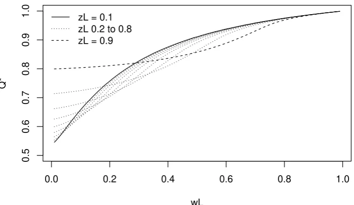
With the optimal excess-spread structure, the quantity of senior securities soldQ∗ exhibits a
more complex relationship to both wLand zL, as shown in Figure 8.
[Figure 8 about here.]
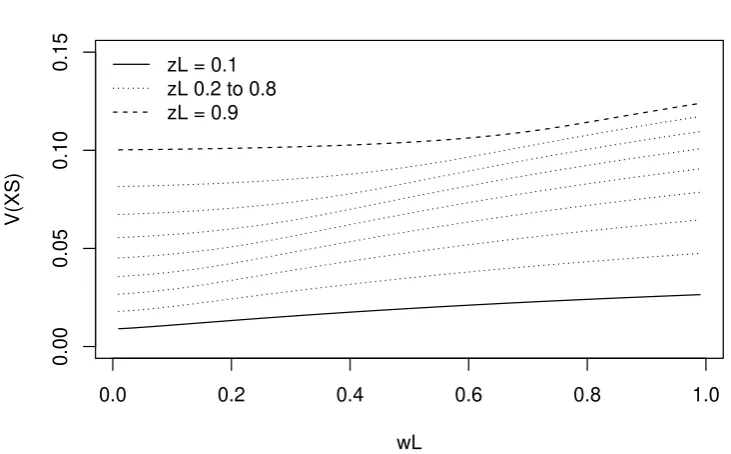
As we have seen in Figure 7, with high-enough wL andzL, the securitization gain to the issuer is
in the order to 0.10. Figure 9 shows that the limiting gain from a NIM resecuritization is fairly
substantial in relation. We can also see that depending onzL, there is a maximum to the value
of a NIM as a function of the worst casewL.
[Figure 9 about here.]
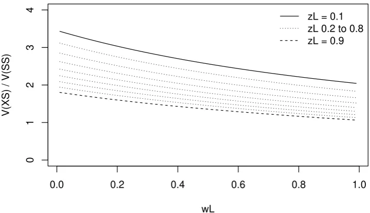
As the minimal recovery declines, and expected losses increase, the value to the issuer of an
excess-spread securitization declines, but Figure 10 shows us that the slope of this decline is
quite small. In effect, the collateral’s coupon increases, for it to be par priced, as expected losses
increase, and the excess-spread structure is able to make use of that higher coupon. A standard
senior/subordination structure is not able to use the extra coupon, and its value to the issuer
declines to a greater extent as expected losses increase.
[Figure 10 about here.]
Looking at the ratio of the value to the issuer of an excess-spread structure to the value of a
standard structure as shown in Figure 10, we can see how par-priced collateral with a low credit
quality will be much more efficiently securitized through an excess-spread structure.
6
Conclusion
Securitization has been a subject of interest in the security design literature, and various models
have been developed in order to explain why such transactions should produce senior securities
and junior securities. However securitization structures are far more complex than a simple
tranching by seniority.
Using a model inspired from the existing literature, specifically DeMarzo and Duffie (1999) and
DeMarzo (2005), we have extended the analysis by considering that interest and principal should
be separately contractible, and that the senior bonds in a securitization should be par-priced.
This allowed us to derive optimal designs closely resembling actual securitization structures.
Further, we showed that the resecuritization of residuals, in the form of NIMs or reremics, was
optimal through a pooling effect comparable to that observed in DeMarzo (2005). Finally, we
carried out a simple numerical analysis when the collateral is priced at par reflecting securitization
execution. This has allowed us to illustrate how important resecuritization is, and also how more
attractive an XS/OC structure was relative to a standard SI/SS as expected collateral losses
increased. According to our analysis, the apparent complexity in excess-spread structure and in
resecuritizations can be explained by a valid optimal design argument.
One important shortcoming in our analysis is that we have not addressed any of the complex
dynamic aspects in securitization structures, as we only considered a two period economy.
Extending security design models to a continuous time framework may make it possible to
account for the optimality of some even more complex mechanisms, such as triggers and the
timing of principal release.
7
Appendix
7.1 Proof of Optimality of Dynamic Debt
Proof. First, since we have assumed Y has a uniform worst-casezL, then using Proposition 10
from DeMarzo and Duffie (1999), we know that among all contracts of the formg(Y), where
interest is not contractible separately, the optimal contract has the formg(Y) =Y ∧D for some
D.
Let us now show that optimal contracts have the formf(x)k(v) = (x∧D0)(v∧D1). We consider
relative to x and v. Given g, we define a dynamic debt contract d(x, v) = (x∧D0)(v∧D1).
Note that as a function ofD1 and as a function of D0, dis increasing and continuous. We set
D0 and D1 such that
E[d(X, V)|Z =zL] =E[g(X, V)|Z =zL].
Finding such values forD0 and D1 is possible sincedis continuous and increasing relative to
them, and varyingD0 andD1, 0≤d(x, v)≤xv, and 0≤g(x, v)≤xv.
Then, comparing V(d(X, V)) and V(g(X, V)) only depends on the difference between
E[d(X, V)|Z] and E[g(X, V)|Z]. We write e(x, v) = g(x, v)−d(x, v), which may be positive or negative, but is continuous in x and in v. In addition, for V ≥D1 and X ≥D0,e(x, v) is
increasing inv. Hence there exists a continuous functionv∗ depending ong,D0 and D1 such
thatv > v∗(x) is equivalent toe(x, v)>0.
Now, we write
E[e(X, V)|Z =z] =E[Ie(X,V)>0e(X, V)|Z =z] +E[Ie(X,V)≤0e(X, V)|Z =z] =E[IV >v∗(X)e(X, V)νz(V)|Z =zL]
+E[IV≤v∗(X)e(X, V)νz(V)|Z =zL],
where we know that νz is increasing. Noting that the second term in the sum is negative, we
can write:
E[e(X, V)|Z =z]≥E[νz(v∗(X))]E[e(X, V)|Z =zL].
However, we setD0 andD1 so thatE[e(X, V)|Z =zL] = 0 and therefore E[e(X, V)|Z =z]≥0.
As a consequence, given a generic contract g, we have determined a superior contract of the
form (x∧D0)(V ∧D1).
Now, we consider contracts of this formg(x, v) =f(x)k(v), with f(x) = (x∧D0) and k(v) =
(v∧D1). We can write
V(g(X, V)) = y
1 +yE[f(X)]E[k(V)|Z =zL]E
E[k(V)|Z =z
L] E[k(V)|Z]
y1
.
This value is maximal for f set as the identity, and therefore the optimal contract takes the
7.2 Conditions for Uniform Worst-Case
Proof. We want to show that AZ has a uniform worst-case zL for any independent random
variableA with distributionµA verifying the conditions in the Proposition.
In this case we can write the conditional expectation E[g(AZ)|Z =z] as follows
Z
g(y)µ(y, z)dy=
Z
g(za)µA(a)da
=
Z
g(y)µA
y z dy z = Z
g(y)zLµA
y z zµA y zL µA y zL dy zL = Z
g(zLa)
zLµA zzLa
zµA(a)
µA(a)da.
And therefore the Radon-Nikodym derivative is
νz(y) =
zLµA yz
zµA
y
zL
.
Since the zLis a lower bound ofZ, any valuez in the domain ofZ verifiesz≥zL and zzL >1.
For νz(y) to be increasing, the first derivative needs to be positive. If we write a = yz and
αa= zy
L for simplicity (with α >1), the condition is:
µ′A(a)µA(αa)≥αµA(a)µ′A(αa).
Now we show that ifµA is log-concave, along with another condition, then the condition
µ′
A(a)
µA(a)
≥αµ
′
A(αa)
µA(αa)
is verified.
Assume that µA is log-concave. In this case µ′
A
µA is decreasing. We also assume the ratios are
defined and vanish at zero, so that µ′A(a)
µA(a) goes to zero when agoes to zero. With a = 0, we
see that this is necessary for the inequality to be verified, otherwise we would arrive to α≤1.
Therefore we see that µ′A
Now, we note that thanks to log-concavity
µ′
A(a)
µA(a)
≥ µ
′
A(αa)
µA(αa)
,
but both sides of this inequality are negative so
µ′
A(αa)
µA(αa)
≥αµ
′
A(αa)
µA(αa)
,
and the condition is verified.
If on the other hand we do not assume that µ′A(a)
µA(a) goes to zero whenagoes to zero, then we need
to assume that µ′A(a)
µA(a) goes to infinity whenagoes to zero, again so thatα ≤1 is not implied. In
this case, µ′A
µA ≥0 at least on some of its domain. In the cases where this quantity is negative, we
can infer the condition as we have above. Where µ′A
µA is positive, andµ
′
Ais positive, the condition
of log-concavity is not sufficient and we need a stronger specific assumption, that:
µ′A(a)
µA(a)
≥αµ
′
A(αa)
µA(αa)
.
This implies that the second derivative of µ′A(a)
µA(a) be negative enough.
Hence, the variables of the form ZAadmit a uniform worst-case equal to infZ whenA has a
log-concave distribution µA either with µ′
A(a)
µA(a) vanishing in zero, or if
µ′ A(a)
µA(a) goes to infinity in
zero, then the stronger condition that µ′A(a)
µA(a) ≥α
µ′ A(αa)
µA(αa) is required.
7.3 Optimality of NIM Securitization
Proof. We follow the outline of the proof of Theorem II in DeMarzo (2005).
We know that V = W Z and Y = XW Z have zL as a uniform worst case, and so does
(ZXW−D∗)IZXW−D∗≥0 as an increasing function. Thanks to the log-concavity assumption,
P
i(ZiXiWi−D∗)IZiXiWi−D∗≥0 also admits a uniform worst-case relative to the Zi and since
the distribution is the same for all iit is equal tozL.
Hence, thanks to Proposition ??we know that among all security designs of the form
g 1 n n X
i≥1
(ZiXiWi−D∗)IZiXiWi−D∗≥0
a standard debt contract
gdN IM
1 n n X
i≥1
(ZiXiWi−D∗)IZiXiWi−D∗≥0
= 1 n n X
i≥1
(ZiXiWi−D∗)IZiXiWi−D∗≥0
∧d
is optimal.
Let us now define
jn(d, z) =E
1 n n X
i≥1
(ZiXiWi−D∗)IZiXiWi−D∗≥0
∧d|∀i≤n:Zi =z =E 1 n n X
i≥1
(zXiWi−D∗)IzXiWi−D∗≥0
∧d
.
As zL is the uniform worst case for all the ZiXiWi we have
inf (zi)1≤i≤n
E 1 n n X
i≥1
(ZiXiWi−D∗)IZiXiWi−D∗≥0
∧d|∀i≤n:Zi =zi
=E 1 n n X
i≥1
(ZiXiWi−D∗)IZiXiWi−D∗≥0
∧d|∀i≤n:Zi=zL
=jn(d, zL).
The value to the issuer of the contract gd
N IM is therefore as follows (we did not write the full
random variable expression on the left-hand side for brevity):
V(gN IMd ) = y
1 +yjn(d, zL)
E
jn(d, zL) Eh1n
Pn
i≥1(ZiXiWi−D∗)IZiXiWi−D∗≥0
∧d|(Zi)1≤i≤n
i 1 y .
The XiWi are independent and identically distributed, so thanks to the weak law of large
numbers, we know that jn(d, z) converges and
lim
n→∞jn(d, z) =E[(zW X−D ∗)