Reducing infrequent-token perplexity via variational corpora
Yusheng Xie1,# Pranjal Daga1
1Northwestern University
Evanston, IL USA
Yu Cheng2
Kunpeng Zhang3
2 IBM Research
Yorktown Heights, NY USA
Ankit Agrawal1 Alok Choudhary1
3 University of Maryland
College Park, MD USA
Abstract
Recurrent neural network (RNN) is recog-nized as a powerful language model (LM). We investigate deeper into its performance portfolio, which performs well on frequent grammatical patterns but much less so on less frequent terms. Such portfolio is ex-pected and desirable in applications like autocomplete, but is less useful in social content analysis where many creative, un-expected usages occur (e.g., URL inser-tion). We adapt a generic RNN model and show that, with variational training cor-pora and epoch unfolding, the model im-proves its performance for the task of URL insertion suggestions.
1 Introduction
Just 135 most frequent words account for 50% text of the entire Brown corpus (Francis and Kucera, 1979). But over 44% (22,010 out of 49,815) of Brown’s vocabulary arehapax legomena1. The
in-tricate relationship between vocabulary words and their utterance frequency results in some impor-tant advancements in natural language process-ing (NLP). For example, tf-idf results from rules applied to word frequencies in global and local context (Manning and Sch¨utze, 1999). A com-mon preprocessing step for tf-idf is filtering rare words, which is usually justified for two reasons. First, low frequency cutoff promises computa-tional speedup due to Zipf’s law (1935). Second, many believe that most NLP and machine learning algorithms demand repetitive patterns and reoc-currences, which are by definition missing in low frequency words.
1.1 Should infrequent words be filtered?
Infrequent words have high probability of becom-ing frequent as we consider them in a larger
con-1Words appear only once in corpus.
text (e.g.,Ishmael, the protagonist name in Moby-Dick, appears merely once in the novel’s dialogues but is a highly referenced word in the discus-sions/critiques around the novel). In many modern NLP applications, context grows constantly: fresh news articles come out on CNN and New York Times everyday; conversations on Twitter are up-dated in real time. In processing online social me-dia text, it would seem premature to filter words simply due to infrequency, the kind of infrequency that can be eliminated by taking a larger corpus available from the same source.
To further undermine the conventional justifica-tion, computational speedup is attenuated in RNN-based LMs (compared ton-gram LMs), thanks to modern GPU architecture. We train a large RNN-LSTM (long short-term memory unit) (Hochreiter and Schmidhuber, 1997) model as our LM on two versions ofJane Austen’s complete works. Deal-ing with 33% less vocabulary in the filtered ver-sion, the model only gains marginally on running time or memory usage. In Table 1.1, “Filtered pus” filters out all the hapax legomena in “Full cor-pus”.
Full corpus Filtered corpus
corpus length 756,273 751,325 vocab. size 15,125 10,177 running time 1,446 sec 1,224 sec GPU memory 959 MB 804 MB
Table 1: Filtered corpus gains little in running time or memory usage when using a RNN LM.
Since RNN LMs suffer only small penalty in keeping the full corpus, can we take advantage of this situation to improve the LM?
1.2 Improving performance portfolio of LM
One improvement is LM’s performance portfo-lio. A LM’s performance is usually quantified as
perplexity, which is exponentialized negative log-likelihood in predictions.
For our notation, let VX denote the vocabu-lary of words that appear in a text corpus X =
{x1, x2, . . .}. Given a sequencex1, x2, . . . , xm−1, where each x ∈ VX, the LM predicts the next in sequence,xm ∈ VX, as a probability distribu-tion over the entire vocabulary V (its prediction denoted as p). If vm ∈ VX is the true token at positionm, the model’s perplexity at index mis quantified asexp(−ln(p[vm])). The training goal is to minimize average perplexity acrossX.
However, a deeper look into perplexity beyond corpus-wide average reveals interesting findings. Using the same model setting as for Table 1.1, Figure 1 illustrates the relationship between word-level perplexity and its frequency in corpus. In general, the less frequent a word appears, the more unpredictable it becomes. In Table 1.2, the trained model achieves an average perplexity of 78 on filtered corpus. But also shown in Table 1.2, many common words register with perplexity over 1,000, which means they are practically un-predictable. More details are summarized in Table 1.2. The LM achieves exceptionally low perplex-ity on words such as<apostr.>s (’s, the posses-sive case), <comma>(, the comma). And these tokens’ high frequencies in corpus have promised the model’s average performance. Meanwhile, the LM has bafflingly high perplexity on common-place words such asreadandconsidering.
64 128 256 512 1024 2048 4096 8192 16384 32768 65536
0 1000 2000 3000 4000 5000 6000 7000 8000 9000 10000
Wo
rd
freq
uen
cy
in
co
rp
us
Wo
rd
level
a
vera
ge p
erp
lexi
ty
word perplexity
word frequency (log scale)
Figure 1: (best viewed in color) We look at word level perplexity with respect to the word frequency in corpus. The less frequent a word appears, the more unpredictable it becomes.
2 Methodology
We describe a novel approach of constructing and utilizing pre-training corpus that eventually reduce LMs’s high perplexity on rare tokens. The stan-dard way to utilize a pre-training corpusW is to
Token Freq. Perplexity 1 Perplexity 2
corpus avg. N/A 78 82
<apostr.>s 4,443 1.1 1.1
of 23,046 4.9 5.0
<comma> 57,552 5.2 5.1
been 3,452 5.4 5.7
read 224 3,658 3,999
quiet 108 6,807 6,090
returning 89 7,764 6,268
considering 80 9,573 8,451
Table 2: A close look at RNN-LSTM’s perplexity at word level. “Perplexity 1” is model perplexity based on filtered corpus (c.f., Table 1.1) and “Per-plexity 2” is based on full corpus.
first train the model onW then fine-tune it on tar-get corpus X. Thanks to availability of text, W
can be orders of magnitude larger thanX, which makes pre-training onW challenging.
A more efficient way to utilizeW is to construct variational corpora based onXandW. In the fol-lowing subsections, we first describe how replace-ment tokens are selected from a probability mass function (pmf), which is built from W; then ex-plain how the variational corpora variates with re-placement tokens through epochs.
2.1 Learn from pre-training corpus
One way to alleviate the impact from infrequent vocabulary is to expose the model to a larger and overarching pre-training corpus (Erhan et al., 2010), if available. Let W be a larger corpus than X and assume that VX ⊆ VW. For exam-ple, if X is Herman Melville’s Moby-Dick, W
can be Melville’s complete works. Further, we useVX,1 to denote the subset ofVX that are ha-pax legonema in corpus X; similarly, VX,n (for
n= 2,3, . . .) denotes the subset ofVX that occur
ntimes inX. Many hapax legomena in VX,1 are likely to become more frequent tokens inVW.
Suppose that x ∈ VX,1. Denoted by ReplacePMF(W, VW, x) in Algorithm 1, we rep-resentxas a probability mass function (pmf) over
{x0
1, x02, . . .}, where eachx0iis selected fromVW∩ VX,n forn > 1using one of the two methods be-low. For illustration purpose, suppose the hapax legomenon,x, in question ismatrimonial:
distance. We set the measure threshold very high (>0.93), which minimizes false positives as well as captures many hapax legonema due to adv./adj., pl./singular (e.g,-y/-ilyand-y/-ies).
2) e.g.,maritalWords that are direct syno/hypo-nyms toxin the WordNet (Miller, 1995).
getContextAround(x0) function in Algorithm 1
simply extracts symmetric context words from both left and right sides of x0. Although the
in-vestigated LM only uses left context in predicting wordx0, context right ofx0is still useful
informa-tion in general. Given a context wordcright ofx0,
the LM can learnx0’s predictability overc, which
is beneficial to the corpus-wide perplexity reduc-tion.
In practice, we select no more than 5 substitu-tion words from each method above. The prob-ability mass on eachx0
i is proportional to its fre-quency in W and then normalized by softmax: pmf(x0
i) = freq(x0i)/P5k=1freq(x0k). This sub-stitution can help LMs learn better because we re-place the un-trainableVX,1tokens with tokens that can be trained from the larger corpusW. In con-cept, it is like explaining a new word to school kids by defining it using vocabulary words in their ex-isting knowledge.
2.2 Unfold training epochs
Epoch in machine learning terminology usually means a complete pass of the training dataset. many iterative algorithms take dozens of epochs on the same training data as they update the model’s weights with smaller and smaller adjust-ments through the epochs.
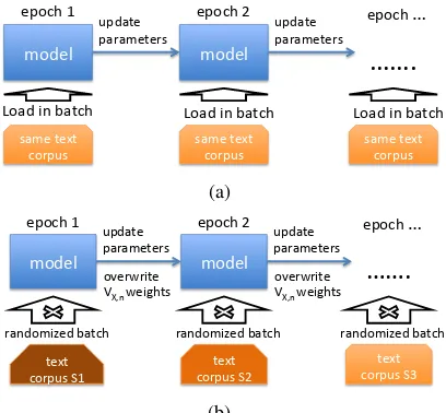
We refer to the the training process proposed in Figure 2 (b) as “variational corpora”. Com-pared to the traditional structure in Figure 2 (a), the main advantage of using variational corpora is the ability to freely adjust the corpus at each ver-sion. Effectively, we unfold the training into sep-arate epochs. This allows us to gradually incorpo-rate the replacement tokens without severely dis-torting the target corpusX, which is the learning goal. In addition, variational corpora can further regularize the training of LM in batch mode (Sri-vastava et al., 2014).
Algorithm 1 constructs variational corpora
X(s)at epochs. AssumingX(s+ 1)being avail-able, Algorithm 1 appends snippets, which are sampled fromW, intoX(s)for thesth epoch. For the last epochs = S,X(S) = X. As the epoch
model&
same&text&& corpus&
Load&in&batch& update& parameters& epoch&1&
model&
same&text&& corpus&
update& parameters& epoch&2&
&…….&
Load&in&batch&
epoch&…&
same&text&& corpus&
Load&in&batch&
(a)
model&
text&& corpus&S1&
randomized&batch& update& parameters&
epoch&1&
&…….&
epoch&…&model&
text&& corpus&S2&
randomized&batch& update& parameters&
epoch&2&
text&& corpus&S3&
randomized&batch& overwrite&
VX,n&weights&
overwrite& VX,n&weights&
[image:3.595.314.518.61.250.2](b)
Figure 2: Unfold the training process in units of epochs. (a) Typical flow where model parses the same corpus at each epoch. (b) The proposed training architecture with variational corpora to in-corporate the substitution algorithm.
Algorithm 1: Randomly constructs varia-tional corpus at epochs.
Input:W, X, VW, VX, VX,n, n, as defined in Section 1.2&2.1,
s, S, current and max epoch number.
Output:X(s), variational corpus at epochs
1 X(s)←X(s+ 1) 2 for eachx∈VX,ndo
3 p←ReplacePMF(W, VW, x)
4 i←Dirichlet(p).generate() 5 whilei←X.getNextIdxOf(x)do 6 x0 ←i.draw()
7 c←W.getContextAround(x0) 8 c.substr(0,uniformRnd 0,S−Ss|c|) 9 X(s).append(c)
10 returnX(s)
number increases, fewer and shorter snippets are appended, which alleviates training stress. By fix-ing annvalue, the algorithm applies to all words inVX,n.
Freq. nofilter 3filter ptw vc
10 28,542 (668.1) 23,649 (641.2) 27,986 (1,067.2) 20,994(950.9) 100 1,180.3 (21.7) 1,158.2 (19.2) 735.8(29.8) 755.8 (31.5) 1K 163.2 (12.9) 163.9 (12.2) 138.5 (14.1) 137.7(15.7) 5K 47.5 (3.3) 47.2 (3.1) 40.2(3.2) 40.2(3.3) 10K 16.4 (0.31) 16.7 (0.29) 14.4 (0.42) 14.1(0.41) 40K 7.6 (0.09) 7.6 (0.09) 7.0(0.09) 7.0(0.10) all tokens 82.1 (2.0) 77.9 (1.9) 68.6(2.1) 68.9 (2.1)
GPU memory 959MB 783MB 1.8GB 971MB
[image:4.595.101.497.61.208.2]running time 1,446 sec 1,181 sec 9,061 sec 6,960 sec
Table 3: Experiments compare average perplexity produced by the proposed variational corpora approach and other methods on a same test corpus. Bold fonts indicate best. “Freq.” indicates the average corpus-frequency (e.g., Freq.=1K means that words in this group, on average, appear 1,000 times in corpus). Perplexity numbers are averaged over 5 runs with standard deviation reported in parentheses. GPU memory usage and running time are also reported for each method.
Err. type Context before True token LM prediction
False neg. <unk>, via,<unk>, banana, muffin, chocolate, URL to a cooking blog recipe
False neg. sewing, ideas,<unk>, inspiring, picture, on, URL to favim.com esty
False neg. nike, sports, fashion,<unk>, women,<unk>, URL to nelly.com macy
False pos. new, york, yankees, endless, summer, tee,<unk>, shop <url>
False pos. take, a, rest, from, your, #harrodssale, shopping <url>
Table 4: False positives and false negatives predicted by the model in the Pinterest application. The context words preceding to token in questions are provided for easier analysis3.
3 Experiments
3.1 Perplexity reduction
We validate our method in Table 3 by showing per-plexity reduction on infrequent words. We split Jane Austen’s novels (0.7 million words) as tar-get corpus X and test corpus, and her contem-poraries’ novels4 as pre-training corpus W (2.7
million words). In Table 3, nofilteris the unfil-tered corpus; 3filter replaces all tokens in VX,3 by<unk>;ptwperforms naive pre-training onW
then onX;vcperforms training with the proposed variational corpora. Our LM implements the RNN training as described in (Zaremba et al., 2014). Ta-ble 3 also illustrates the GPU memory usage and running time of the compared methods and shows thatvcis more efficient than simplyptw.
vc has the best performance on low-frequency words by some margin.ptwis the best on frequent words because of its access to a large pre-training
3Favim.com is a website for sharing crafts, creativity
ideas. Esty.com is a e-commerce website for trading hand-made crafts. Nelly.com is Scandinavia’s largest online fash-ion store. Macy’s a US-based department store. Harrod’s is a luxury department store in London.
4Dickens and the Bronte sisters
corpus. But somewhat to our surprise, ptw per-forms badly on low-frequency words, which we reckon is due to the rare words introduced inW: while pre-training on W helps reduce perplexity of words inVX,1but also introduces additional ha-pax legomena inVW,1\VX,1.
0 0.1 0.2 0.3 0.4 0.5
tech animals travel food home fashion
Ac
cu
ra
cy
nofilter 3filter ptw vc
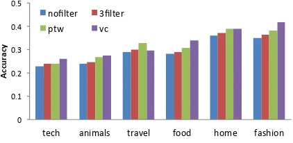
Figure 3: Accuracy of suggested URL positions across different categories of Pinterest captions.
3.2 Locating URLs in Pinterest captions
[image:4.595.311.522.526.629.2]site (Linder et al., 2014; Zhong et al., 2014). To maximally preserve user experience, postings on Pinterest embed URLs in a natural, nonintrusive manner and a very small portion of the posts con-tain URLs.
In Figure 3, we ask the LM to suggest a po-sition for the URL in the context and verify the suggest with test data in each category. For ex-ample, the model is presented with a sequence of tokens: find, more, top, dresses, at, afford-able, prices,<punctuation>, visit, and is asked to predict if the next token is an URL link. In the given example, plausible tokens aftervisitcan be either <http://macys.com> or nearest, Macy,
<apostr.>s, store. The proposedvc mechanism outperforms others in 5 of the 6 categories. In Figure 3, accuracy is measured as the percentage of correctly suggested positions. Any prediction next to or close to the correct position is counted as incorrect.
In Table 4, we list some of the false nega-tive and false posinega-tive errors made by the LM. Many URLs on Pinterest are e-commerce URLs and the vendors often also have physical stores. So in predicting such e-commerce URLs, some mis-takes are “excusable” because the LM is confused whether the upcoming token should be an URL (web store) or the brand name (physical store) (e.g,http://macys.comvs.Macy’s).
4 Related work
Recurrent neural network (RNN) is a type of neu-ral sequence model that have high capacity across various sequence tasks such as language model-ing (Bengio et al., 2000), machine translation (Liu et al., 2014), speech recognition (Graves et al., 2013). Like other neural network models (e.g., feed-forward), RNNs can be trained using back-propogation algorithm (Sutskever et al., 2011). Recently, the authors in (Zaremba et al., 2014) successfully apply dropout, an effective regular-ization method for feed-forward neural networks, to RNNs and achieve strong empirical improve-ments.
Reducing perplexity on text corpus is proba-bly the most demonstrated benchmark for mod-ern language models (n-gram based and neural models alike) (Chelba et al., 2013; Church et al., 2007; Goodman and Gao, 2000; Gao and Zhang, 2002). Based on Zipf’s law (Zipf, 1935), a fil-tered corpus greatly reduces the vocabulary size
and computation complexity. Recently, a rigor-ous study (Kobayashi, 2014) looks at how per-plexity can be manipulated by simply supplying the model with the same corpus reduced to vary-ing degrees. Kobayashi (2014) describes his study from a macro point of view (i.e., the overall corpus level perplexity). In this work, we present, at word level, the correlation between perplexity and word frequency.
Token rarity is a long-standing issue with n -gram language models (Manning and Sch¨utze, 1999). Katz smoothing (Katz, 1987) and Kneser-Ney based smoothing methods (Teh, 2006) are well known techniques for addressing sparsity in
n-gram models. However, they are not directly used to resolve unigram sparsity.
Using word morphology information is another way of dealing with rare tokens (Botha and Blun-som, 2014). By decomposing words into mor-phemes, the authors in (Botha and Blunsom, 2014) are able to learn representations on the morpheme level and therefore scale the language modeling to unseen words as long as they are made of previ-ously seen morphemes. Shown in their work, this technique works with character-based language in addition to English.
5 Acknowledgements
This work is supported in part by the following grants: NSF awards CCF-1029166, IIS-1343639, and CCF-1409601; DOE award DESC0007456; AFOSR award FA9550-12-1-0458; NIST award 70NANB14H012.
6 Conclusions & future work
This paper investigates the performance portfolio of popular neural language models. We propose a variational training scheme that has the advan-tage of a large pre-training corpus but without us-ing as much computus-ing resources. On low fre-quency words, our proposed scheme also outper-forms naive pre-training.
In the future, we want to incorporate WordNet knowledge to further reduce perplexity on infre-quent words.
References
probabilistic language model. Journal of Machine
Learning Research, 3:1137–1155.
Jan A. Botha and Phil Blunsom. 2014. Compositional morphology for word representations and language
modelling. InProceedings of the 31th International
Conference on Machine Learning, ICML 2014,
Bei-jing, China, 21-26 June 2014, pages 1899–1907.
Ciprian Chelba, Tomas Mikolov, Mike Schuster, Qi Ge, Thorsten Brants, Phillipp Koehn, and Tony Robin-son. 2013. One billion word benchmark for measur-ing progress in statistical language modelmeasur-ing. Tech-nical report, Google.
Kenneth Church, Ted Hart, and Jianfeng Gao. 2007. Compressing trigram language models with golomb
coding. In EMNLP-CoNLL 2007, Proceedings
of the 2007 Joint Conference on Empirical Meth-ods in Natural Language Processing and Compu-tational Natural Language Learning, June 28-30,
2007, Prague, Czech Republic, pages 199–207.
Dumitru Erhan, Yoshua Bengio, Aaron Courville, Pierre-Antoine Manzagol, Pascal Vincent, and Samy Bengio. 2010. Why does unsupervised pre-training
help deep learning? J. Mach. Learn. Res., 11:625–
660, March.
Nelson Francis and Henry Kucera. 1979. Brown cor-pus manual. Technical report, Department of Lin-guistics, Brown University, Providence, Rhode Is-land, US.
Jianfeng Gao and Min Zhang. 2002. Improving lan-guage model size reduction using better pruning
cri-teria. In Proceedings of the 40th Annual Meeting
on Association for Computational Linguistics, ACL
’02, pages 176–182, Stroudsburg, PA, USA. Associ-ation for ComputAssoci-ational Linguistics.
Joshua Goodman and Jianfeng Gao. 2000. Language model size reduction by pruning and clustering. In Sixth International Conference on Spoken Language Processing, ICSLP 2000 / INTERSPEECH 2000,
Beijing, China, October 16-20, 2000, pages 110–
113.
Alex Graves, Abdel-rahman Mohamed, and Geof-frey E. Hinton. 2013. Speech recognition with
deep recurrent neural networks. In IEEE
Interna-tional Conference on Acoustics, Speech and Signal Processing, ICASSP 2013, Vancouver, BC, Canada,
May 26-31, 2013, pages 6645–6649.
Sepp Hochreiter and J¨urgen Schmidhuber. 1997. Long
short-term memory. Neural Comput., 9(8):1735–
1780, November.
S. Katz. 1987. Estimation of probabilities from sparse data for the language model component of a speech
recognizer. Acoustics, Speech and Signal
Process-ing, IEEE Transactions on, 35(3):400–401, Mar.
Hayato Kobayashi. 2014. Perplexity on reduced
cor-pora. InProceedings of the 52nd Annual Meeting of
the Association for Computational Linguistics
(Vol-ume 1: Long Papers), pages 797–806. Association
for Computational Linguistics.
Rhema Linder, Clair Snodgrass, and Andruid Kerne. 2014. Everyday ideation: all of my ideas are on
pinterest. InCHI Conference on Human Factors in
Computing Systems, CHI’14, Toronto, ON, Canada
- April 26 - May 01, 2014, pages 2411–2420.
Shujie Liu, Nan Yang, Mu Li, and Ming Zhou. 2014. A recursive recurrent neural network for statistical
machine translation. InProceedings of the 52nd
An-nual Meeting of the Association for Computational
Linguistics (Volume 1: Long Papers), pages 1491–
1500, Baltimore, Maryland, June. Association for Computational Linguistics.
Christopher D. Manning and Hinrich Sch¨utze. 1999. Foundations of Statistical Natural Language
Pro-cessing. MIT Press.
Tomas Mikolov, Ilya Sutskever, Kai Chen, Gregory S. Corrado, and Jeffrey Dean. 2013. Distributed rep-resentations of words and phrases and their
compo-sitionality. InNIPS, pages 3111–3119.
George A. Miller. 1995. Wordnet: A lexical database
for english. Commun. ACM, 38(11):39–41,
Novem-ber.
Razvan Pascanu, Tomas Mikolov, and Yoshua Bengio. 2013. On the difficulty of training recurrent neural
networks. InProceedings of the 30th International
Conference on Machine Learning, ICML 2013,
At-lanta, GA, USA, 16-21 June 2013, pages 1310–1318.
Nitish Srivastava, Geoffrey Hinton, Alex Krizhevsky, Ilya Sutskever, and Ruslan Salakhutdinov. 2014. Dropout: A simple way to prevent neural networks
from overfitting. Journal of Machine Learning
Re-search, 15:1929–1958.
Ilya Sutskever, James Martens, and Geoffrey Hinton. 2011. Generating text with recurrent neural net-works. In Lise Getoor and Tobias Scheffer, editors, Proceedings of the 28th International Conference
on Machine Learning (ICML-11), ICML ’11, pages
1017–1024, New York, NY, USA, June. ACM. Yee Whye Teh. 2006. A bayesian interpretation of
interpolated kneserney. Technical report.
Wojciech Zaremba, Ilya Sutskever, and Oriol Vinyals.
2014. Recurrent neural network regularization.
arXiv preprint arXiv:1409.2329.
Changtao Zhong, Mostafa Salehi, Sunil Shah, Mar-ius Cobzarenco, Nishanth Sastry, and Meeyoung Cha. 2014. Social bootstrapping: how pinterest and last.fm social communities benefit by borrowing
links from facebook. In 23rd International World
Wide Web Conference, WWW ’14, Seoul, Republic
G.K. Zipf. 1935. The Psycho-biology of Language:
An Introduction to Dynamic Philology. The MIT