On the neural substrates of the disposition effect and return performance

Munich Personal RePEc Archive

On the neural substrates of the

disposition effect and return performance

Dorow, Anderson and Da Costa Jr, Newton and Takase,

Emilio and Prates, Wlademir and Da Silva, Sergio

2017

On the neural substrates of the disposition effect

and return performance

Anderson Dorow

_{Newton Da Costa Jr}

_{, Emilio Takase}

Wlademir Prates

_{Sergio Da Silva}

a_{Graduate Program in Management, Federal University of Santa Catarina, Florianopolis, SC,}

88040-900, Brazil

b_{School of Business, Pontifical Catholic University of Parana, Curitiba, PR, 80215-901, Brazil}

c_{Department of Psychology, Federal University of Santa Catarina, Florianopolis, SC, 88040-970,}

Brazil

d

Graduate Program in Economics, Federal University of Santa Catarina, Florianopolis, SC, 88040-900, Brazil

* _{Corresponding author. Tel.: +55 48 3721 9901; fax: +55 48 3721 9901. Email address:}

[email protected] (S. Da Silva).

Abstract

We experimentally assess the disposition effect and return performance, using electroencephalogram to measure the brain activity of the participants. The design of the experiment follows a previous protocol (Frydman et al., 2014). Our sample was made up of 12 undergraduates (all male, age range 18 to 29, mean age 22.2) and five professional stock traders (all male, age range 21 to 37, mean age 30.2). We find neural support for the finding that professionals are more likely to escape the disposition effect (Da Costa Jr et al., 2013). We also find higher heart rate variability and brainwave activation are positively related to stock returns. Electrical activity tends to increase with returns, mainly for the beta waves that are activated in conscious states.

Subject areas: neurofinance,behavioral finance

Keywords: disposition effect, neurofinance, beta electric brain wave, psychophysiology

Data availability:The authors confirm that all data underlying the findings are fully available without restriction by request. The dataset is posted at Figshare (https://dx.doi.org/10.6084/m9.figshare.4312091.v1).

Funding: Research was funded by CNPq (Conselho Nacional de Desenvolvimento Científico e Tecnológico, Bolsa de Produtividade em Pesquisa). The funder had no role in study design, data collection, and analysis, decision to publish, or preparation of the manuscript.

Competing interests: The authors have declared that no competing interests exist.

Ethical committee approval: The research received approval from the Ethical Committee for Research on Human Beings of the Federal University of Santa Catarina (case number:1.744.242; date of approval: September 26, 2016).

1. Introduction

In current economics and finance, bounded rationality is an assumption of financial behavior that coexists with that of full rationality. Historically, full rationality was challenged by the experimental discoveries initiated in the 1980s within the research on behavioral finance (Heukelom, 2014). One such well-documented finding was the disposition of stock traders for selling winners rather than losers. The anomaly has received an opaque label: the disposition effect. That is, the disposition to sell winners too early and ride losers too long (Shefrin and Statman, 1985). The discovery meant investors are reluctant to realize their losses (Odean, 1998). Many explanations have been proposed but none is established. An obvious account that can be accommodated with full rationality is plain mean reversion. An investor keeps losing stocks just because he or she rationally guesses the stocks will gain in value in the future. However, bounded rationality is more generally accepted to lie at the heart of the disposition effect. Here, there are many hypotheses that share the understanding of the disposition effect as a cognitive bias. “Prospect theory” was an early candidate, but even its proponent now favors the so-called “narrow framing hypothesis” (Kahneman, 2011). An investor sets up an account for each share he or she bought, and wishes to close every account as a gain. The rationale of mental accounting is bounded because a full rational attitude is to consider the portfolio as a whole and sell the stock that is more likely to underperform in the future, regardless of whether it is a winner or a loser.

The neural substrates of financial biases, such as the disposition effect, can be assessed by the complementary, emerging field of neurofinance (Sahi, 2012). Neurofinance examines experimentally the nature of the cognitive processes engaged in acquiring and processing information in financial decision making. Financial decisions are analyzed by applying neurotechnology to observe and understand neural traits affecting trading and their possibly associated biases. Neurofinance assumes investors have different psychophysiological make-ups, and these can affect the investors’ ability to make full rational decisions in investing (Tseng, 2006).

The neural data coming from neurofinance experiments can be helpful in testing models of investor behavior (Frydman et al., 2014). A recent study confirmed the disposition effect is due to bounded rationality, but not of the narrow framing type (Frydman et al., 2014).The authors conducted the study in an experimental market where participants traded stocks while their brain activity was measured using functional magnetic resonance imaging (fMRI). There emerged neural evidence that investors derive utility directly from realizing gains and losses on the sale of stocks they own, in addition to deriving utility from consumption (a hypothesis called “realization utility” (Barberis and Xiong, 2009)). Importantly, the neural data also cast doubt on the mean reversion hypothesis.

Here, we experimentally reassess the disposition effect adopting the neurofinance perspective (Frydman et al., 2014), but measure brain activity with electroencephalogram (EEG) rather than fMRI. EEG is usually employed to track electrical activity in the brain. Brain cells communicate with each other through electrical impulses and an EEG test can record them. Thus, EEG detects brain wave patterns. Further, we consider the disposition effect at the behavioral level as well as the neural level (Frydman et al., 2014). And we also try to replicate previous findings regarding the disposition effect at the psychophysiological level (Goulart et al., 2013). Our study is nuanced by the distinction we make between professional investors and amateurs. At the behavioral level, professionals were shown more likely to escape the disposition effect (Da Costa Jr et al., 2013), a result that receives neural support from our experimental data.

Despite being published as recently as 2014, the paper of Frydman et al. has already received 90 citations, including ours. Using their evidence that investors trade based on a specific portion of wealth in

finding that the best and worst-ranked positions are more likely to be sold compared to positions in the middle of the portfolio. However, it has been warned that discontinuity tests on U.S. investor trades do not support sign realization preference, and show that it is not the source of the disposition effect (Hirshleifer, 2015; Ben-David and Hirshleifer, 2012). Moreover, Clarke (2014) criticizes the neurofinance approach of Frydman et al. (2014) on methodological grounds by pointing to a simple modus tollens, disrupting their argument. Their first premise is that an economic model entails a specific cognitive hypothesis. One then learns, using neurofinance data, that the cognitive hypothesis is false. So, one must conclude that the content of the economic model is also false. However, because economic models of decision making do not entail specific cognitive hypotheses when they are construed appropriately, the first premise of the above argument is false (Clarke, 2014). Rather than aiming to prove or disprove alternative explanations of the disposition effect, here we only investigate whether it emerges in our neural data, regardless of the mechanism that generates it.

The next section presents the materials and methods of our study; Section 3 displays the results found; and Section 4 concludes the report.

2. Materials and methods

2.1 Participants and sample

We assembled a sample of 12 undergraduates (all male, age range 18 to 29, mean age 22.2) and five professional traders (all male, age range 21 to 37, mean age 30.2). The students came from the Federal University of Santa Catarina, Florianopolis, in southern Brazil. They were undergraduates enrolled in economics, accounting or management. The professionals also came from the Florianopolis area. This seems like a small sample for behavioral studies, but for most neuro studies it cannot be considered uncommon because, it is argued, adding more participants usually does not seem to alter results a great deal (Bhatt and Camerer, 2005). The participants were all right-handed, had no history of psychiatric illness and none were taking medication. The students reported no previous financial market experience. Homogenizing the sample according to these characteristics provides reliability concerning the particular results generated from the neuro and physiological output. The downside is that the sample is hardly random. Instead, the behavior of the participants is likely to overstate that of a random population. All the participants read the purpose of the experiment and then signed a term of consent. The research received approval from the Ethical Committee for Research on Human Beings of the Federal University of Santa Catarina (case number: 1.744.242; date of approval: September 26, 2016). The dataset is available at Figshare (https://dx.doi.org/10.6084/m9.figshare.4312091.v1).

The sessions for data collection were conducted at the Brain Education Lab at the Federal University of Santa Catarina, under the supervision of the lab director (author E.T.). The sessions took place during the morning and the chronotype characteristics of the participants were thus ignored. The room temperature was kept constant at 24 degrees Celsius. Prior to the sessions, the experimenter (author A.D.) gave a questionnaire to collect information regarding age and whether the participant had previous experience with stock trading, whether he was taking medication, and whether he has a history of illness or brain damage. The session durations ranged 15 to 60 minutes.

2.2 Measuring neural activity

neurofeedback and biofeedback system for real-time data acquisition in a clinical or research setting. We used the channel appropriate for viewing the EEG and concentrated on the alpha and beta brainwaves. We only considered data with 100 percent quality signals.

The communication between neurons within our brains underlies all our thoughts and emotions. Synchronized electrical pulses from neurons communicating with each other produce brainwaves that can be detected using sensors placed on the scalp. The brainwaves are divided into bandwidths to describe a continuous spectrum of consciousness: from slow, loud and functional to fast, subtle and complex. Brainwave speed is measured in hertz (Hz), which means cycles per second. The brainwaves change according to what one is doing and feeling. In particular, alpha waves (8 to 12 Hz) occur during quietly flowing thoughts and refer to the resting state of the brain. Alpha waves help mental coordination, calmness, alertness and learning. Beta waves (12 to 38 Hz) are present in the normal waking state of consciousness when one is alert, attentive, and focused on problem solving, judgment, and decision making.

The equipment was equipped with a 60 Hz filter that automatically removed electrical interference from the room’s electric power. ProComp Infiniti offers no risk of electrical shocks.

2.3 Measuring heart rate activity

We measured the heart rate using the EKG (electrocardiogram) channel of the ProComp Infiniti equipment.Normal heart rate produces four waves: a P wave, a QRS complex, a T wave and a U wave. The P wave represents atrial depolarization; the QRS complex represents ventricular depolarization; the T wave represents ventricular repolarization; and the U wave represents papillary muscle repolarization. In particular, the QRS complex corresponds to the depolarization of the right and left ventricles. It normally lasts from .06 to 10 seconds. The Q, R and S waves occur in succession and reflect a single event. A Q wave is a downward deflection after the P wave. An R wave follows as an upward deflection, and the S wave is a downward deflection after the R wave. The T wave follows the S wave. In some situations, an extra U wave follows the T wave.

One of the variables we measured was the RR interval, that is, the time interval in milliseconds between two R waves. Our choice is justified by the fact that the RR interval produces a peak of energy higher than the others produce, and is thus more visible on the EKG. We also considered as a separate variable the square root of the mean squared differences between successive RR intervals. In addition, another variable we considered was the standard deviation of successive RR intervals, which is thought to track the parasympathetic nervous system activity.

2.4 Design of behavioral task

The behavioral task followed closely that in Frydman et al. (2014). First, we developed an open source software (called Investor) to simulate the stock market. Investor was designed purposefully to test the disposition effect in connection with the ProComp Infiniti equipment. Investor generates an output of the trade decisions of each participant, and thus computes the disposition effect according to the formulas to be presented in Section 2.6. Investor also simultaneously records the alpha and beta waves along with the heart rate every period using the input received from the ProComp Infiniti equipment.

professional trader) or one point on the final exam of the course from which the student participant was recruited. Giving course points to students is an almost perfect substitute to giving them cash (Moore and Taylor, 2007).

The experimental instructions were shown on the first screen of Investor. The screen then flicked and a second screen informed: 1) which stock had been randomly selected (whether stock A, B or C); 2) the purchase price of the selected stock in the experimental currency; and 3) the current price of the stock relative to its purchase price, an information that allowed a participant to evaluate whether the stock had gained in value or not.

After two seconds, the second screen flicked and a blank screen was shown for 1.3 seconds. This is the time span required for the neurobiofeedback equipment to get ready and track the subsequent decision, which was made on the fourth screen. This screen displayed the trade choice the participant had to make. In addition to repeating the second-screen information, the participant was now shown his cash balance and then asked if he wanted to buy, sell or hold the stock. The participant had to make this decision within a five-second timespan. Whenever a decision was not made within this period, a random one was made by the software (Figure 1). We chose the five-second decision timespan based on feedback from a pilot experiment designed to find the smallest span of time necessary for a decision in this context. Our choice of five seconds agrees with previous vindication (Engelmann et al., 2009; Horlings, 2008), but not with the choice of three seconds made in Frydman et al. (2014).

Figure 1. Investor’s screens presented to the participants.

screen displays of each of the three stocks were random, there was no reason for one participant to expect pattern. In particular, the random price path of each stock was governed by a two-state Markov chain with a good state and a bad state. The Markov chain for each stock was independent of the Markov chains for the other two stocks (Frydman et al., 2014). Finally, the actual experiment resumed during the subsequent 21 trials.

We also imposed further restrictions (Frydman et al., 2014) as follows. 1) One participant had to hold a maximum of one share and a minimum of zero shares of each stock (A, B or C) at any trial. 2) Short selling was not allowed, only the selling of a stock currently held in the portfolio. 3) Transactions of fractions of shares were not allowed. 4) Purchase of a stock for a price above the current cash balance was allowed, which means a negative cash balance could occur temporarily. 5) Temporary negative cash balances were subtracted from the final return. (Further details of the behavioral task have been omitted because it closely mimicked that in Frydman et al. (2014).)

2.5 Simulation

Prior to each session, a participant sat in front of a desktop PC running the software Investor and five electrodes of the ProComp Infiniti equipment were posted on a participant’s skin following standard protocol (Teplan, 2002). Voluntary movements, such as scratching, chatting and sudden gestures, generate artifacts that should be removed from the sample (Teplan, 2002). So a participant was instructed to stay seated, prevent sudden gestures during the session, breathe normally, and also not to chat or ask questions (Teplan, 2002).

The instructions were presented in verbal form (lasting two minutes on average) and then again in text on the Investor’s first screen. This aimed to assure everyone received the same instructions (Costa‐ Gomes et al., 2001; Friedman and Sunder, 1994). The experimenter then collected the neurological and physiologicalbaseline of a participant in a state of rest. An accurate baseline is a critical benchmark from which to compare the subsequent neurophysiological signals (Camerer et al., 2005).

To get real involvement of the participants in the experiment, they were primed by a story where they were told they were the only provider for a family of five and, crucially, their performance in the coming experiment would affect the family’s success to survive and thrive. This priming aimed at guaranteeing homogeneous expectations and common targets for the participants (Benz and Meier, 2008).

2.6 Measuring the disposition effect and return performance

We considered the most usual measure of the disposition effect (Odean, 1998). In a given period, each stock was assigned to one of four categories: 1) As a “realized gain,” whenever it was sold at a price that was higher than the average purchase price. 2) As a “realized loss,” whenever it was sold at a price that was lower than the average purchase price. 3) As a “paper gain,” whenever its price was higher than its average purchase price, but it was not sold during that period. And 4),as a “paper loss,” whenever its price was lower than its average purchase price, but it was not sold during that period. The “proportion of gains realized” (PGR) reckons the number of gains realized as a fraction of the number of gains that could have been realized. It is then

total number of realized gains PGR

total number of realized gains total number of paper gains



 . (1)

total number of realized losses PLR

total number of realized losses total number of paper losses



 . (2)

The disposition effect occurs if PGR > PLR. For example (Odean, 1998), PGR = .148 and PLR = .098. Whenever the difference between PGR and PLR is greater than .76, the realization utility hypothesis predicts a burst of utility in the brain (Frydman et al., 2014; Barberis and Xiong, 2009).

To assess the statistical significance of the disposition effect, we employed the usual Z test for the differences of proportion, as follows:

   

PGR PLR

PGR 1 PGR PLR 1 PLR

total number of realized gains total number of paper gains total number of realized losses total number of paper losses

Z 

 



 

. (3)

This conventional measure of the disposition effect (Odean, 1998) is the one considered in Frydman et al. (2014). One problem is that we are left with only 17 observations for each participant. For this reason, we further considered the total of purchases and sellings of each participant, which renders us with an enlarged sample of 164 observations. This alternative metric (Grinblatt and Keloharju, 2001; Barberis and Huang, 2001; Kaustia, 2010) uses a logistic regression, and fits well for incorporating the neurophysiological variables. Moreover, by considering it, we are also able to track return performance.

We estimated the propensity of participant i to sell or not a stock and, as a result, realize a gain or a loss in time step t. We assessed the influence of large and small returns, both positive and negative. We first modeled the influence of large returns (intervals [ 10, 5]  and [5,10] ), two brainwave variables (B1

and B₂), three heart rate variables (H₁, H₂, and H₃), and status of a participant S (whether professional investor or not) on the propensity to sell (Y 1) or not (Y 0) the stock:

0 1 [ 10, 5] 2 [5,10] 3 1 4 2 5 3 6 1 7 2 8

it it it it it it it it it it it it it it it it it it it

Y       H  H  H  B  B  S u , (4)

where H₁ tracks the RR interval, that is, the time interval in milliseconds between two R waves; H₂ is the square root of the mean squared differences between successive RR intervals; H3 is the standard

deviation of successive RR intervals; B₁ is the beta wave; B₂ is the alpha wave; and u is an error term. A similar model was estimated for small returns (intervals [ 5,0] and [0,5] ):

0 1 [ 5, 0] 2 [0,5] 3 1 4 2 5 3 6 1 7 2 8

it it it it it it it it it it it it it it it it it it it

Y      H  H  H  B  B  S u . (5)

Large and small returns were separated to prevent collinearity problems.

In addition, we considered logit regressions to estimate the propensity to sell versus to hold a stock (Grinblatt and Keloharju, 2001; Kaustia, 2010). The dependent variable takes the value of one for sales, and zero for holds.

3. Results

thus confirming previous literature (Da Costa Jr et al., 2013). The result was statistically significant (t test = 10.19, p <.01; two-tailed Mann-Whitney U test = 28.1831, p < .001). The professionals also beat the students regarding return performance (15.6 percent versus 4.1 percent).

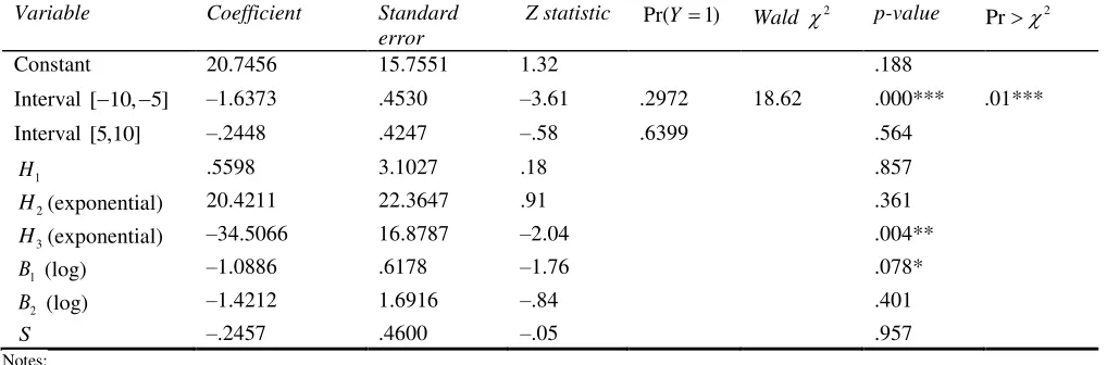
As for return performance, Table 1 shows the results by considering the influence of large returns (intervals [ 10, 5]  and [5,10] ) (equation (4)). Negative values show an inverse relationship between the probability of success of the dependent variable and the independent variable.

Table 1. Estimates of equation (4)

Variable Coefficient Standard

error

Z statistic Pr(Y 1) Wald 2 p-value ( Pr2

Constant 20.7456 15.7551 1.32 .188

Interval [ 10, 5]  ‒1.6373 .4530 ‒3.61 .2972 18.62 .000*** .01***

Interval [5,10] ‒.2448 .4247 ‒.58 .6399 .564

1

H .5598 3.1027 .18 .857

2

H (exponential) 20.4211 22.3647 .91 .361

3

H (exponential) ‒34.5066 16.8787 ‒2.04 .004**

1

B (log) ‒1.0886 .6178 ‒1.76 .078*

2

B (log) ‒1.4212 1.6916 ‒.84 .401

S ‒.2457 .4600 ‒.05 .957

Notes:

Number of observations with Y0: 72 Number of observations with Y 1: 95

Total number of observations of the logistic regression: 164 Hausman log-likelihood test = ‒100.8539

*significant at 10 percent; **significant at 5 percent; *** significant at 1 percent

Table 2 shows the results by considering the influence of small returns (intervals [ 5, 0] and [0,5]) (equation (5)).

Table 2. Estimates of equation (5)

Variable Coefficient Standard

error

Z statistic Pr(Y 1) Wald 2 p-value ( Pr2

Constant 19.9516 15.9571 1.25 .211

Interval [ 5, 0] .3316 .4059 .82 .5355 .414 .03**

Interval [0,5] 1.6533 .4861 3.40 .8119 .001***

1

H ‒.1912 3.1462 ‒.06 .952

2

H (exponential) 20.8183 22.3422 .93 .351

3

H (exponential) ‒34.3831 16.6298 ‒2.07 .039**

1

B (log) ‒1.0178 .6043 ‒1.68 .092**

2

B (log) ‒1.4974 1.6879 ‒.89 .375

S ‒.1712 .4524 ‒.38 .705

Notes:

Number of observations with Y0: 72 Number of observations with Y 1: 95

Total number of observations of the logistic regression: 164 Hausman log-likelihood test = ‒101.6387

The results in Table 1 for large returns show the propensity to sell is smaller within the negative interval, while for small returns in Table 2 the propensity to sell is greater (0.81). Both results combined suggest the presence of the disposition effect. Moreover, the results in Tables 1 and 2 are in line with prospect theory. Prospect theory predicts the propensity to sell a stock declines as its price moves away from the purchase price in either direction (Kaustia, 2010).

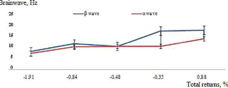
The results in Tables 1 and 2 also suggest higher heart rate variability and brainwave activation are positively related to returns. Figure 2 shows electrical activity tends to increase with returns, mainly for beta waves. Previous literature has found professionals are not conscious of the impact of historical returns on their expectations (Kaustia et al., 2008). However, this seems at odds with our finding of a correlation between beta waves and returns.

Figure 2. Brainwaves and returns are positively correlated.

Conclusion

Our main contribution in this paper is to experimentally reassess the disposition effect adopting the neurofinance perspective while measuring brain activity with electroencephalogram (EEG). This adds to the existing neurofinance studies that gauges brain activity using fMRI, such as that of Frydman et al. (2014). Further, we consider the disposition effect at the behavioral and psychophysiological level as well as the neural level. In addition, our study is nuanced by the distinction we make between professional investors and amateurs. At the behavioral level, we provide neural support for the literature result (Da Costa Jr. et al., 2013) that professionals are more likely to escape the disposition effect. Importantly, our key result is to find that higher heart rate variability and brainwave activation are positively related to returns. Electrical activity tends to increase with returns mainly for the beta waves that are activated in conscious states. This holds true for both large and small returns.

References

Barberis N, Huang M (2001) Mental accounting, loss aversion, and individual stock returns. Journal of Finance 56 (4), 1247-1292.

Barberis N, Xiong W (2009) What drives the disposition effect? An analysis of a long-standing preference-based explanation.

Journal of Finance 64 (2), 751-784.

Ben-David I, Hirshleifer D (2012) Are investors really reluctant to realize their losses? Trading responses to past returns and the disposition effect. Review of Financial Studies 25 (8), 2485-2532.

Benz M, Meier S (2008) Do people behave in experiments as in the field? Evidence from donations. Experimental Economics

11 (3), 268-281.

Bhatt M, Camerer CF (2005) Self-referential thinking and equilibrium as states of mind in games: fMRI evidence. Games and Economic Behavior 52 (205), 424-459.

Camerer C, Loewenstein G, Prelec D (2005) Neuroeconomics: How neuroscience can inform economics. Journal of Economic Literature 43 (1), 9-64.

Clarke C (2014) Neuroeconomics and confirmation theory. Philosophy of Science 81 (2), 195-215.

Costa‐Gomes M, Crawford VP, Broseta B (2001) Cognition and behavior in normal‐form games: An experimental study.

Econometrica 69 (5), 1193-1235.

Da Costa Jr N, Goulart M, Cupertino C, Macedo Jr J, Da Silva S (2013) The disposition effect and investor experience. Journal of Banking & Finance 37 (5), 1669-1675.

Engelmann JB, Capra CM, Noussair C, Berns GS (2009) Expert financial advice neurobiologically “offloads” financial

decision-making under risk. PLoS ONE 4 (3), e4957.

Friedman D, Sunder S (1994) Experimental Methods: A Primer for Economists. Cambridge: Cambridge University Press.

Frydman C, Barberis N, Camerer C, Bossaerts P, Rangel A (2014) Using neural data to test a theory of investor behavior: An application to realization utility. Journal of Finance 69 (2), 907-946.

Goulart M, Da Costa Jr N, Santos A, Takase E, Da Silva S (2013) Psychophysiological correlates of the disposition effect.

PLoS ONE 8 (1), e54542.

Grinblatt M, Keloharju M (2001) What makes investors trade? Journal of Finance 56 (2), 589-616.

Hartzmark SM (2015) The worst, the best, ignoring all the rest: The rank effect and trading behavior. Review of Financial Studies 28 (4), 1024-1059.

Heukelom F (2014) Behavioral Economics: A History. New York: Cambridge University Press.

Hirshleifer D (2015) Behavioral finance. Annual Review of Financial Economics 7, 133-159.

Horlings R (2008) Emotion recognition using brain activity. Department of Mediamatics Delft University of Technology Thesis.

Kahneman D (2011) Thinking, Fast and Slow. New York: Farrar, Straus and Giroux.

Kaustia M, Alho E, Puttonen V (2008) How much does expertise reduce behavioral biases? The case of anchoring effects in stock return estimates. Financial Management 37 (3), 391-411.

Moore A, Taylor M (2007) Experimental economics research: Is there an alternative to having huge research budgets?

Economics Bulletin 3 (4), 1-6.

Odean T (1998) Are investors reluctant to realize their losses? Journal of Finance 53 (5), 1775-1798.

Sahi SK (2012) Neurofinance and investment behavior. Studies in Economics and Finance 29 (4), 246-267.

Shefrin H, Statman M (1985) The disposition to sell winners too early and ride losers too long: Theory and evidence. Journal of Finance 40 (3), 777-790.

Teplan M (2002) Fundamentals of EEG Measurement. Measurement Science Review 2 (2), 1-11.