Numerical Investigation on High Performance Supercritical Airfoil using Co Flow Jet Control

915

©IJRASET: All Rights are Reserved

Numerical Investigation on High Performance

Supercritical Airfoil using Co-Flow Jet Control

S. Ragul1, S. Periyasamy2 1

PG Scholar, Department of Thermal Engineering, Government College of Technology, Coimbatore-641013, Tamilnadu, India 2

Assistant Professor, Department of Mechanical Engineering, Government College of Technology, Coimbatore-641013, Tamilnadu, India

Abstract: An airfoil is a cross section of a wing which can create more lift with less drag than any other shapes. Huge Passenger airplanes like Airbus A380 uses supercritical airfoil for its wing design because of its higher critical mach number. This project is based on the increasing lift and reducing drag coefficients by injection of air over the supercritical airfoil surface. The original airfoil was analyzed for the various angles of attack 0, 3, 6 and 9 degrees. From the analysis, the values of the lift and the drag coefficients for the various angles of attack and the minimum pressure point location were obtained. The original airfoil modified with the injection slots at the upper surfaces and the four modified airfoils were obtained. The four modified airfoils were named as model 1, model 2, model 3 and model 4. All the modified airfoils were analysed for the various angles of attack and various injection velocities 100 m/s, 150 m/s and 200 m/s and the results were tabulated. To perform such analysis, the turbulence model k-ε standard wall function was used in the FLUENT. From the analysis, the model 1 gives the high lift coefficient and the low drag coefficient.

Keywords: Co-flow jet, Drag coefficient, Lift coefficient, Minimum pressure point, Supercritical airfoil.

I. INTRODUCTION

An airfoil is the very basic shape in creating an aircraft which has the capability of producing lift with less drag due to its high coefficient of lift and low coefficient of drag value than any other shapes. The airfoil will be considered as the heart of an aircraft. The airfoil directly affects many parameters such as cruise speed, take-off and landing distances, stall speed, coefficient of lift, coefficient of drag and overall aerodynamic efficiency during all phases of flight.

The front of the airfoil is defined by a leading-edge radius which is tangent to the upper and lower surfaces. An airfoil modeled to operate in a supersonic flow will have a sharp or nearly sharp leading edge to prevent a drag producing bow shock.

Usually, all cambered airfoils have larger upper surface than the lower one. That’s the reason it can create lift even at zero degree angle of attack. It’s because the flow over the airfoil need to cover a large distance than the flow on lower surface which causes high velocity at upper surface. According to the Bernoulli’s principle, this increase in velocity will reduce pressure on upper surface and hence a pressure gradient will be created between the lower and upper surfaces of the airfoil that results in lift in a supercritical airfoil, at almost 80% of upper surface is flat such that a high camber will be present at the trailing edge region to create the required lift. This flatness is the reason for its ability to increase the critical mach number value.

Critical mach number is the mach number at which mach value reaches 1 at any point on the airfoil surface, even though the free stream mach number will be less than 1. The reason is the acceleration of free stream flow on the upper surface of the airfoil. Drag divergence mach number is the mach number value at which there will be a tremendous increase in drag value of an airfoil because of the shock wave created above the airfoil surface.

Supercritical airfoils have flattened upper surface than any other airfoils which are used for the aircrafts. Supercritical airfoil and other airfoils may have the same mach number but the drag divergence mach number will be higher for a supercritical airfoil than any other airfoils. That is, a supercritical airfoil can fly at mach number higher than critical mach number before the drag divergence may have been encountered. Because of that, such airfoils are modeled to fly above the critical mach number and hence the name Supercritical airfoil. [5].

The high-performance airfoil should have a combination of maximum coefficient of lift and minimum coefficient of drag. The high performance for the airfoil can be obtained by use of co flow jet control [1,2,3]. The conventional CFJ has both injection slot and suction slot near the leading edge and trailing edge respectively. It utilizes tangentially injected air near the leading edge and tangentially removed air at the trailing edge to increase lift and reduce drag.

916

©IJRASET: All Rights are Reserved

II. MODELLING

The supercritical airfoil that is used for the analysis is the NASA SC (2) 0610, which is shown in Fig. 1. The chord length was taken as 1 m for further calculation and analysis. This airfoil is widely used in Airbus A380 which is very much heavier compared to other passenger aircraft. The airfoil is designed using the ANSYS 17.5 - Design Modeler.

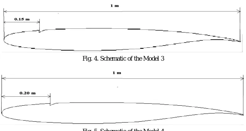
From the analysis, the minimum pressure point is identified at 0.05 % of the chord length. There are four models, named as model 1, model 2, model 3 and model 4. In model 1, the injection slot is placed at 0.05 m from the leading of the airfoil as shown in Fig. 2. The shape and the dimensions of injection slot are also mentioned in Fig. 2. Similar to this, the injection slots are placed at 0.10 m, 0.15 m, and 0.20 m for model 2, model 3 and model 4 respectively. These models are shown in the Figs. 3-5 respectively. The distance of the injection slot for the different models are given in Table 1.

Table 1 Distances of the injection slot for the different models

Name of the Models Distance from the Leading edge in

(m)

Model 1 0.05

Model 2 0.10

Model 3 0.15

Model 4 0.20

Fig. 1. Schematic of the NASA SC (2) 0610 Airfoil

Fig. 2. Schematic of the Model 1

917

©IJRASET: All Rights are Reserved

Fig. 4. Schematic of the Model 3

Fig. 5. Schematic of the Model 4

III. MESHING

In order to analyze fluid flow, the flow domains are split into smaller sub domains. The governing equations were then discretized and solved inside each of the sub domains. The mesh was generated using ANSYS 17.5 – FLUENT. The clustering was made in which the grid size increased from airfoil surface to wall gradually. The fine mesh was applied near the airfoil surface to obtain accurate results. The enclosure was created as shown in Fig. 6.

In order to give the better flow alignment, the C-type grid was used. The front and the back edge of the enclosure were considered to be an inlet and an outlet. In order to give the better flow field, the following distances were considered. The distance between the inlet and the leading edge, the outlet and the trailing edge, the upper edge and the chord, the lower edge and the chord were taken as 15 m respectively. The distance between the outlet and the trailing edge was taken as 25 m.

The distance between the inlet and the L.E is lesser than the distance between the outlet and the T.E. Because, the formation of the wake and the reverse flow ahead of the airfoil is very less when compared to aft the airfoil for the given flow condition. At the same time, the distance between the inlet and the leading edge in the enclosure determines the evenness of the flow ahead of the airfoil. These physics were considered for selecting the above-mentioned distances.

The meshes were controlled by the sizing and the mapped face meshing. In mesh sizing, the behaviour of the mesh was soft and growth rate was 1.2 with no bias conditions. In this mapped face meshing, the method of quadrilaterals was selected. The resulting mesh contained 151926 cells. The minimum and the maximum number of cell sizes are 0.006 m and 0.677950 m. Maximum skewness is 0.784 which is less than 1 and hence the cell quality is good.

918

©IJRASET: All Rights are Reserved

IV. ANALYSIS

First of all, the original airfoil was analyzed at 120 m/s of free stream velocity without injection of flow for the following angles of attack 0, 3, 6 and 9 degrees. Then all the modified airfoils were analyzed at the various angles of attack and the various injection velocities of 100 m/s, 150 m/s and 200 m/s with same magnitude of free stream velocity. After these analyses, the required model was obtained.

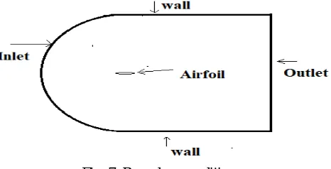
Fig. 7. Boundary conditions

The simulation of the injection flow was done by the Fluent CFD software. The boundary conditions for the analysis is shown in Fig. 7. For the analysis, the 2D analysis was chosen. The flow was steady flow with density based in which the flow is independent of time and compressibility effects are accounted. The Reynolds number was more than 500000 and hence the flow was turbulent flow, in which the fluid particles move in an unpredictable path that results in rapid and continuous mixing of the fluid leading to momentum transfer as flow occurs. Also, it will affect the fluctuation in the velocity and pressure at any point in the flow field. To describe the effect of fluctuations, the suitable turbulence model was selected. The two equation k-ε

turbulence model was selected. It is well suitable for external flows and capable of predicting separated flow than other models. In defining material, air was chosen as fluid and aluminium was chosen as material for both the original and modified airfoils. In boundary condition, the airfoil was given by stationary wall with no slip condition. The injection velocity was 100 m/s and the free stream velocity was 120 m/s. In Inlet and Injection, direction and magnitude method was selected and the angle of attack was zero. The supercritical airfoil can be operated at lower subsonic velocities. Hence the selected freestream velocity gives the required characteristics of supercritical airfoil.

The wall was given by specified shear of zero. The type of outlet was pressure outlet. In defining interference value, the sea level air conditions were selected. In defining the solution control, the courant number was selected as 2, which is used to describe how fluid was moving through your computational cells. Also, the lift and drag coefficients were selected to monitor the lift and drag. Now the iteration was started to reach a constant value. After that the results were noted.

The above mentioned procedure was for model 1 with the injection velocity of 100 m/s and free stream velocity of 120 m/s at zero angle of attack. For the same magnitude of the injection velocity, the angle of attack and the magnitude of free stream velocity, the analyses were done for model 2, model 3 and model 4. The same analytical procedure was used to analyze the all models for various injection velocities of 100 m/s, 150 m/s, 200 m/s at various angles of attack with free stream velocity of 120 m/s and the results were noted. From these analyses, the model 1 gave the better aerodynamic performance than other airfoils and it was selected.

A. Reynolds Number Calculation

Reynolds number, Re= ρ*v*c

µ where,

Density, ρ =1.225 kg/

Velocity, v = 120 m/s

Dynamic viscosity, µ =1.7895* kg/(m.s)

Chord length, c = 1 m Reynolds number, Re = 8214585

919

©IJRASET: All Rights are Reserved

Table 2 Solver setup

Parameter Description

Analysis type 2D-Steady flow with density based

Turbulence model k- ε standard wall function

Fluid type Air

Airfoil surface No slip condition

Wall surface Stationary wall with specified shear of zero

Inlet “Magnitude and direction” method of

velocity inlet

Free stream velocity (m/s) 120

Injection velocities (m/s) 100,150 and 200

Angles of attack (degrees) 0, 3, 6 and 9

Outlet Pressure outlet

Free stream condition Standard Sea level condition

Courant number 2

V. RESULTS

All those analysis of the original and the modified airfoil were done to observe the effect of the flow injection over the airfoil. To perform such comparison, basic parameters are needed. In this project, Static pressure, Coefficient of lift and drag of the airfoils were taken as such basic parameters.

The contours of static pressure for the original and modified airfoils for the various injection velocities at the various angles of attack with the free stream velocity of 100 m/s are shown in Figs. 8-11. The lowest pressure region above the airfoil surface and the minimum pressure were compared to evaluate the effective model.

For the original airfoil, the and values are given in Table 3. These results were compared with those values of and of various models with various injection velocities which were tabulated in Table 4.

To compare the changes of and of the airfoils, the results are plotted as Coefficient of lift vs. Angle of Attack, Coefficient of drag vs. Angle of Attack and Coefficient of lift vs. Coefficient of drag (drag polar). These plots were used to determine the effective model by injection of air in proper position and also to find out the effect of different injection velocities on airfoil parameters.

A. Comparison Of Static Pressure

The Fig. 8 shows the static pressure for the original airfoil at angle of attack of zero degree with free stream velocity of 120 m/s. The leading edge is the stagnation point for any airfoil. The static pressure in the stagnation point is very high compared to other locations on the airfoil surface. Also, due the propagation of pressure, the region near the stagnation pressure has high static pressure compared to other places but lesser than the pressure in the stagnation point.

920

©IJRASET: All Rights are Reserved

The static pressure in the minimum pressure point is very less when compared to other locations on the airfoil. The region near the minimum pressure is also low when compared to other regions. The static pressure decreases from the stagnation point to minimum pressure point which means that negative pressure gradient occurs in between these two points on the upper surface of the airfoil. After the minimum pressure point, the static pressure increases till the trailing edge which means that the positive pressure gradient takes place. Also, the pressure increases in the normal direction to the airfoil surface. The increase in pressure takes in a layer by layer manner which is shown in Fig. 8. But in the actual condition, the increase in a pressure takes place in a particle by particle manner. The lift generation in the supercritical airfoil is mainly due to the high camber in the trailing edge. Hence the pressure in this region is higher than the pressure in the other places of the lower surfaces.

The lift increases with the increase in angle of attack until the stall occurs. The angle of attack considered in this project is less than the stall angle of attack of 13.6 degree. Hence the lift increases with the increase in angle of attack. The lift increases is identified by the reduction in minimum pressure or the lower pressure region above the airfoil surface that is caused by the pressure variation above the airfoil surface.

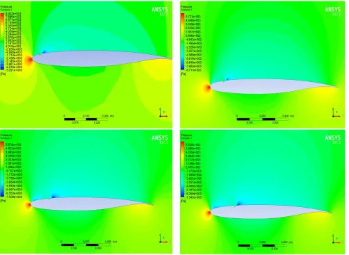
Fig. 9 shows the contours of static pressure of modified airfoils for 100 m/s of injection velocity at angle of attack of 0 degree with freestream velocity of 120 m/s. The model 1 gives the least minimum static pressure compared with the original airfoil at angle of attack of 0 degree and freestream velocity of 120 m/s. Hence lift generated in the model 1 is higher than the original airfoil. But the minimum static pressure of model 1 is higher than the other model for the same flow conditions. However, the model 1 provides the lowest pressure regions above the airfoil surface compared to the other modified airfoils, which leads to high lift generation of model 1 compared to the other models. This can be identified from Fig. 9. Similar to this, the lowest pressure regions above the airfoil surface with the highest minimum pressure occurs for the model 1 compared to the other models at the angle of attack of 3, 6 and 9 degrees.

921

©IJRASET: All Rights are Reserved

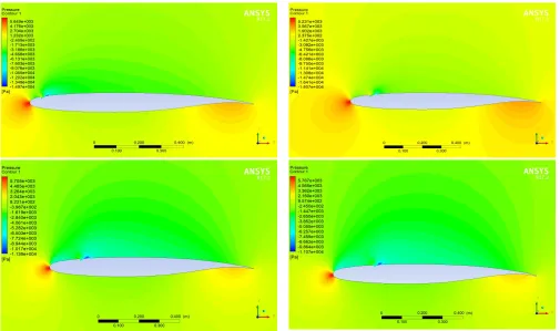
Fig. 10. The contours of static pressure of model 1, model 2, model 3 and model 4 for 150 m/s of injection velocity at zero angle of attack with freestream velocity of 120 m/s

922

©IJRASET: All Rights are Reserved

Fig. 10 shows the contours of static pressure of modified airfoils for 150 m/s of injection velocity at zero angle of attack with freestream velocity of 120 m/s. Similar to the modified airfoils subjected to 100 m/s of injection velocity and same flow conditions, the model 1 provides the least minimum pressure compared to the original airfoil and the lowest pressure region compared to the other modified airfoils for the injection velocity of 150 m/s and same flow conditions. But the minimum pressure is further reduced below the minimum pressure at the injection velocity of 100 m/s for the same flow conditions. Also, the modified airfoils subjected to the injection velocity of 150 m/s provides the lowest pressure region compared to the modified airfoils subjected to 100 m/s for the same flow conditions. This can be identified from the Fig. 10. Similar to this, the lowest pressure regions with the highest minimum pressure occurs at the angle of attack of 3, 6 and 9 degrees.

Fig. 11 shows the contours of static pressure of modified airfoils for 200 m/s of injection velocity at zero angle of attack with freestream velocity of 120 m/s. The injection velocity of 200 m/s provides the least minimum pressure and the lowest pressure regions compared to the other injection velocities for any model at the corresponding angle of attack and the free stream velocity. Also, the model 1 provides lowest pressure region and the least minimum pressure compared to the other modified airfoils and original airfoil for the given flow condition. From the analyses, it is observed that the model 1 gives the lowest pressure region than original airfoil and modified airfoil for the given flow condition. Also, the model 1 gives the least minimum pressure than original airfoil for the given flow condition. It is found that the model 1 is effective than other models. Also, it can be identified from the comparison of lift and drag coefficients.

B. Comparison of Lift and Drag Coefficients

The and are directly proportional to the lift and drag forces respectively. Hence comparing these coefficients of various airfoils directly compares the lift and drag forces of various airfoils.

Table 3 Lift and Drag coefficients of NASA SC (2) 0610 supercritical airfoil for various angles of attack

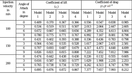
Table 4 Lift and Drag coefficients of different models with various injection velocities and angles of attack Angle of Attack in

degree

Coefficient of lift (cl)

Coefficient of drag (cd)

0 0.3652 0.0098

3 0.4866 0.0175

6 0.6184 0.0537

9 0.7390 0.0921

Injection velocity in m/s Angle of Attack in degree

Coefficient of lift ( )

Coefficient of drag

( )* Model 1 Model 2 Model 3 Model 4 Mode1 1 Model 2 Model 3 Model 4 100

0 0.409 0.370 0.367 0.366 0.556 0.547 0.838 0.985

3 0.534 0.519 0.511 0.507 2.013 2.064 2.447 2.605

6 0.672 0.667 0.665 0.656 4.289 4.352 4.613 4.664

9 0.780 0.775 0.771 0.767 6.992 7.167 8.081 8.798

150

0 0.431 0.402 0.393 0.388 0.336 0.436 0.783 0.798

3 0.564 0.541 0.535 0.528 1.617 2.067 2.431 2.581

6 0.707 0.693 0.687 0.679 4.317 4.473 4.648 4.699

9 0.826 0.821 0.815 0.808 7.222 7.452 7.812 7.986

200

0 0.474 0.442 0.438 0.430 0.226 0.132 0.555 0.605

3 0.616 0.587 0.583 0.577 1.629 1.908 2.235 2.253

6 0.765 0.738 0.734 0.729 4.242 4.513 4.747 4.799

923

©IJRASET: All Rights are Reserved

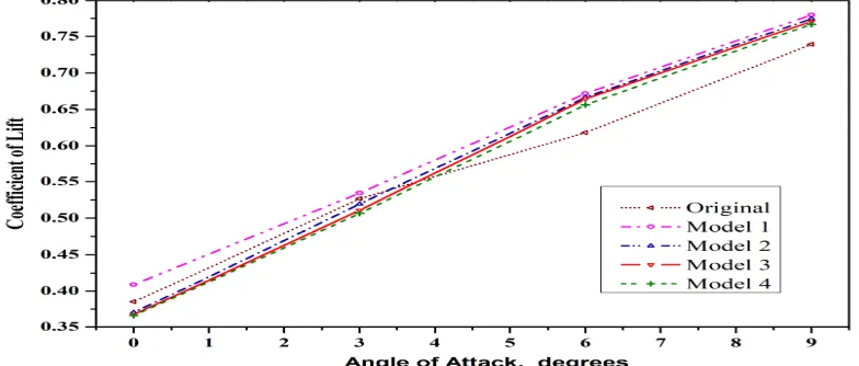
Fig.12 shows the Coefficient of Lift vs. Angle of Attack for the original airfoil and the modified airfoils with injection velocities of 100 m/s. The coefficient of lift increases with increase in angle of attack until the stall occurs. Here the angles of attack were considered less than the angle of attack at stall of 13.6 degree. Hence the coefficient of lift for all the airfoils such that the original and the modified airfoils increase with the increase in angle of attack.

Fig. 12. Coefficient of Lift vs. Angle of Attack for the original and the modified airfoils with Injection velocity of 100 m/s

Fig. 13. Coefficient of Lift vs. Angle of Attack for the original and the modified airfoils with Injection velocity of 150 m/s

924

©IJRASET: All Rights are Reserved

In Fig. 12, the change in coefficient of lift with respect to change in angle of attack which is known as lift curve slope remains more or less constant in between the angles of attack of 0 to 3 degrees and 6 to 9 degrees for the original airfoil. But the lift curve slope is changed and decreased in between 3 to 6 degrees for the original airfoil. However, the lift curve slope for the modified airfoils remain constant for all the given angles of attack with slight variation. The variation of lift curve slope for all the airfoils at the various injection velocities of 150 m/s and 200 m/s also have the similar manner to that of the injection velocity at 100 m/s. But the values of increases with the increase in injection velocities for all the given angles of attack.

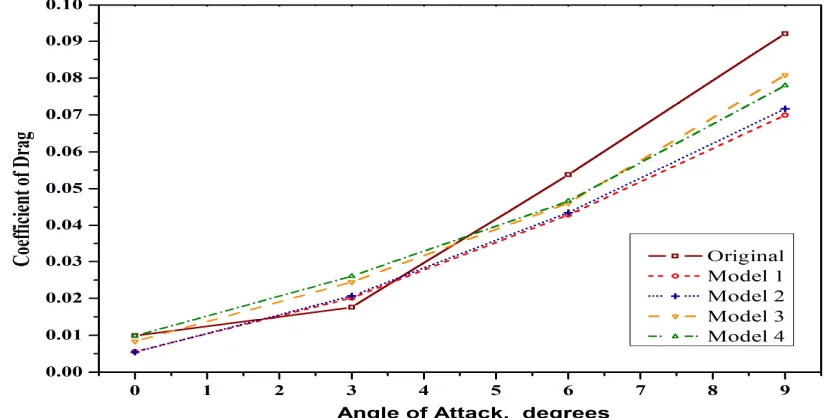
The Coefficient of Lift vs. Angle of Attack for the original airfoil and the modified airfoils with injection velocities of 150 m/s and the 200 m/s are shown in the Figs 13-14 respectively. From these three graphs, it is found that the coefficient of lift at any angles of attack and injection velocities is maximum for the model 1 when compared to the other modified airfoils and the original airfoil. In spite of increment in Coefficient of lift, change in Coefficient of drag plays a major role in selecting the performance of an airfoil. Fig. 15 shows the Coefficient of drag vs. Angle of Attack for the original airfoil and the modified airfoils with the injection velocity of 100 m/s. The coefficient of drag increases with increase in the angle of attack. Hence the coefficient of drag for all the airfoils increase with the increase in angle of attack.

Fig. 15. Coefficient of drag vs. Angle of Attack for the original and the modified airfoils with injection velocity of 100 m/s

925

©IJRASET: All Rights are Reserved

Fig. 17. Coefficient of drag vs. Angle of Attack for the original and the modified airfoils with injection velocity of 200 m/s

In Fig. 15, the Coefficient of drag value of the original airfoil is maximum at zero angle of attack compared to the modified airfoils. But the value of the original airfoil is minimum at the angle of attack of 3 degree compared to the model 2, model 3 and model 4. Because, the change in with respect to the change in angle of attack of original airfoil is minimum compared to all the modified airfoils up to the angle of attack of 3 degree. However, the value is lowest for model 1 at the angle of attack of 3 degree though it has the high change in to the change angle of attack.

After the angle of attack of 3 degree, the value of original airfoil increases rapidly than the modified airfoils for the given change in the angle of attack. Hence the for all the modified airfoil is less than the of the original airfoil in between the angles of attack of 3 to 9 degrees. Also, the reduces with the increase in injection velocity for the given angle of attack. The Coefficient of drag vs. Angle of Attack for the original airfoil and the modified airfoils with injection velocities of 150 m/s and the 200 m/s are shown in the Figs. 16-17 respectively. From these three plots, it is found that at any angles of attack and injection velocities is minimum for the model 1 when compared to the other modified airfoils and the original airfoil. This clearly states that the model 1 is the efficient model for better aerodynamic performance in creating high lift with less drag.

926

©IJRASET: All Rights are Reserved

Also, the graph is plotted between Coefficient of lift vs. Coefficient of drag to clearly identify this physics. The Coefficient of lift vs. Coefficient of drag for the injection velocities of 100 m/s, 150 m/s and 200 m/s are shown in the Figs. 18-20 respectively. In Fig. 18, the of the modified airfoils is higher than the of the original airfoil for the given up to the angle of attack of 3 degree. After the angle of attack of 3 degree, the of the modified airfoils are lower than the of the original airfoils for the given . Comparing all the airfoils for the injection velocity of 100 m/s, the model 1 provides the minimum for the given after the angle of attack of 3 degree. Also, for the injection velocities 150 m/s and 200 m/s, the model 1 provides the minimum for the given at all the angles of attack. This clearly shows that the model 1 has the maximum with minimum . Hence model 1 provides the high aerodynamic performance.

Fig. 19. Coefficient of lift vs. Coefficient of drag for the original and modified airfoils with the injection velocity of 150 m/s

Fig. 20. Coefficient of lift vs. Coefficient of drag for the original and modified airfoils with the injection velocity of 200 m/s

VI. CONCLUSION

927

©IJRASET: All Rights are Reserved

REFERENCES

[1] Abdul Khalid sheriff, J., AjithKumar, A., Karlmarkx, G.K.P., Ashish jayandar, R. and Manikandan, S. (2014) ‘Co-Flow Jet Control as an Alternative for Civil Aircraft High Lift Configuration’, International Journal of Mechanical and Production Engineering, ISSN: 2320-2092, Volume- 2.

[2] Riajun Noor, Md., Assad-Uz-Zaman, Md. (2014) ‘Effect of Co-Flow Jet over an Airfoil: Numerical Approach’ Contemporary Engineering sciences, Vol. 7, no.17, 845.

[3] Gecheng Zha, Sebastian Aspe, Joseph John Dussling, Nicholas Ramsay Heinz and Martinez, Daniel.J. (2008) ‘CoFlow Jet Aircraft’, US 2009/0014592 A1 -United States Patent.