Online Full Text



Abstract— Temporal data mining techniques are important

addition to the field of demand forecasting and stock optimization especially in health applications like drug stock optimization in public clinics. Optimizing drug stock amounts saves a substantial amount of money while maintaining the same level of health service. This paper introduces an enhancement of the temporal pattern matching algorithm as one of the temporal data mining techniques. The enhancement is in the form of replacing the human intuition in selecting the patterns being matched (against the last pattern of arbitrary length of the investigated time series) by systematically searching for them in historical data. The search process is done by applying time series motif discovery algorithm to obtain the set of most similar patterns to the last pattern in the time series. The proposed algorithm also integrates an outlier removal procedure to overcome the expected dispersion of the forecast values due to the probable big number of returned patterns from the motif discovery step. These additions to the temporal pattern matching algorithm improve the quality of patterns being matched and improve the overall forecasting accuracy. The key idea of our algorithm is that it simultaneously performs the pattern matching task – as a necessary step for demand forecasting – while discovering the most similar patterns in historical data. The proposed algorithm is useful if the investigated drug is new and does not have a long enough history to make demand forecast using the ordinary statistical methods. Experimental results show that the time series prediction using this method is more accurate than the traditional prediction methods especially in the cases of new drugs that do not have enough history to make future consumption prediction.

Index Terms— motif discovery, stock optimization, temporal

pattern matching, time series prediction

I. INTRODUCTION

PTIMIZING drug stock amounts in family health units is an important topic from the economic and health perspectives especially in developing countries like Egypt where both issues are important and it is not acceptable to solve one issue in favor of the other. The unnecessary accumulated drugs in public clinics’ pharmacies represent an economic waste of valuable resources and increase the chances of drug expiration; on the other hand, the shortage of stock of certain drugs (due to inability to predict

accu-Mohamed A. El-Iskandarani is a professor of computer science at the Institute of Graduate Studies and Research (IGSR), Alexandria University, 163 Horreya Avenue, El-Shatby 21526 , P.O. Box 832, Alexandria, Egypt. Phone: +201001296350; Fax: +2034285792; e-mail: ([email protected] ).

Saad M. Darwish is an Associate Professor of computer science at the IGSR, Alexandria, Egypt, (e-mail: [email protected]).

Marwan A. Hefnawy is a M.Sc. researcher at the IGSR, Alexandria, Egypt, and is a data analyst in the MoHP, Egypt; (e-mail: [email protected] ).

rately the near future needs in advance) may lead to drug shortage and health problems in the community.

Many prediction techniques are there for time series depending on the assumption that the future trends of data can be predicted from its history. However, in applications like drugs demand forecasting there may be sudden change in the pattern of the time series due to an epidemic for example. Also, the health authorities may replace some drugs that have a long recorded history with new brands for many reasons; in this case there is no available history for the new drugs in order to predict its future consumption. These situations follow pre-defined patterns rather than following the past history of the same time series.

Time series forecasting techniques can be classified generally into three categories: statistical, decomposition, and artificial intelligence techniques [1]-[4]. Statistical tech-niques such as Auto Regression and Moving Average are characterized with their simplicity but they assume that the time series is stationary and have a priori behavior. De-composition methods such as Fourier deDe-composition are powerful in decomposing time series into multiple periodic time series components and the forecast will be made upon each component. Artificial intelligence methods’ accuracy differs according to the nature of the problem, its dataset and the used accuracy performance measures. Neural Networks as one of the AI methods is more flexible because it fore-casts stationary and non-stationary time series and is model free, but it requires a big amount of historical data to be well trained.

A distinct technique for time series forecasting based on matching the last pattern of the time series against other known historical patterns was introduced in [1]. It solves the problem of predicting time series that have very short history which cannot be predicted using the above men-tioned forecasting methods. The authors of [1] remarked two advantages of their forecasting method versus the traditional time series forecasting methods: (1) their forecasting tech-nique does not require a significant amount of historical data to build and train the prediction model and (2) unlike the traditional methods, their technique can predict the turning point and detect sudden behavioral changes. The pattern matching component in this forecasting technique focuses on matching the beginning of many historical patterns against the end of the targeted time series. The aim of this match is to decide if a known pattern from the history is repeated at the time series’ end and which pattern (or a combination of patterns) the time series will most likely follow. However, this approach neglects how to discover these patterns from the history of the same time series (if exists) or from the history of other time series of similar products. The concept of motif discovery in time series

Drug Consumption Prediction through Temporal

Pattern Matching

Mohamed A. El-Iskandarani , Saad M. Darwish, Marwan A. Hefnawy

compensates the shortage of how to discover patterns in the time series before matching them.

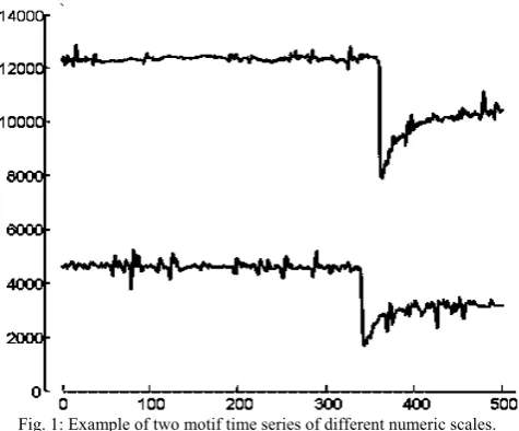
Time series motifs are defined as pairs of individual time series, or subsequences of a longer time series, which are very similar to each other as illustrated in Fig.1. The process of discovering motifs in time series is extracting previously unknown recurrent patterns from time series data. This process could be used as a subroutine in other data mining tasks including prediction, discovering association rules, clustering and classification [5],[6],[7]. Motif discovery has many applications in various areas like detecting patterns in data measured from the human brain, stock prices analysis [8].

Discovering motifs in time series can be divided into two categories [5],[7],[9]: (1) probabilistic and (2) exact. Proba-bilistic motif discovery depends on representing all the sub-sequences of the time series into a collision matrix using some kind of representation. Each similar pair of this repre-sentation is added to the collision matrix as a suspected motif. The largest entries are examined on their original data to decide if they are motifs or not. The advantage of proba-bilistic motif discovery is its robustness to noise and it can find all the motifs with high probability after a certain number of iterations. However, it uses several parameters that need to be tuned. These parameters can be optimized only by experimentation, which is most of the time unfeasible for large datasets. Failing to achieve optimal parameter values in probabilistic motif discovery can lead to misleading results such as: no motifs found, a massive number of motifs or meaningless motifs being found [9]. On the other hand, the algorithm of exact motif discovery de-scribed in [5] has advantages over the methods of proba-bilistic motif discovery in terms of the accuracy of the discovered motifs and the speed performance. It uses initially the brute force searching with all possible pairs of subsequences and enhances the performance by applying the notion of early abandoning the Euclidean Distance calcula-tion when the current cumulative sum is greater than the best-so-far [9].

In our proposed technique, we will apply the speeded up brute force motif discovery algorithm presented in [5] to identify the top k motifs for the last pattern with arbitrary length of the time series. The top k motifs are being

searched within the consumption history of the same (or related) drug in the same (or other) clinics. The resultant top

k motifs are used as input for the dynamic pattern matching technique described in [1] to predict the near future drug demand. This technique is mainly useful when the short history prior to the point of estimation of a time series follows standard known patterns from the same time series or from a time series representing the consumption of another related drug (even if the patterns have different numeric scales).

The remainder of this paper is as follows: Section 2 ex-plains preliminaries that formally define the problem at hand. Section3 contains literature survey of time series fore-casting methods. Section 4 introduces the proposed tech-nique for forecasting drug demand in details. Section 5 reports the accuracy and performance evaluation of the proposed technique and gives experimental results. Finally, section 6 summarizes the conclusion and future work.

II. PRELIMINARIES

This section defines the key terms used in the process of motif discovery and the proposed forecasting technique: Definition 1: A Time Series is a sequence , . . , , which is an ordered set of n real valued numbers. The ordering is temporal [8].

Definition 2: A Time Series Database (D) is an unordered set of m time series. We assume in our work that D fits in the main memory. We can think of D as a matrix of real values where its ith _{row is the time series T}

i and Di,j is the

value at time j of Ti [5].

Definition 3: The Time Series Motif of a time series database D is the unordered pair of time series {Ti, Tj} in D

which is the most similar among all possible pairs. More formally, ∀a,b,i,j the pair {Ti, Tj} is the motif if and only if , , , i ≠ j and a ≠ b. The i ≠ j and a

≠ b are used to exclude the trivial case of considering the time series as a motif with itself. The distance between two time series , is the z-normalized Euclidean distance [5].

Definition 4: The kth-Time Series motif is the kth most similar pair in the database D. The pair {Ti, Tj} is the kth

motif if and only if there exists a set S of pairs of time series of size exactly k-1 such that ∀ ∈ , ∉

, ∉ ∀ Tx,Ty ∈S, Ta,Tb ∉ S

dist Tx,Ty ≤ dist Ti,Tj ≤dist (Ta,Tb) [5].

Definition 5: A subsequence of length q of a time series , . . , is a time series , , . . , for

1 1 [8].

2.1 Problem Definition:

Objective:

Given a time series , , … , of arbitrary length

n, we need to forecast it with arbitrary length f, i.e. we need to get , , … , .

Inputs:

 A univariate time series S of length n where each point represents a certain clinic’s consumption of a certain drug in one month.

 The last subsequence in S of arbitrary length w definedas

, , … . , where .

 An arbitrary integer f that represents length of the output forecast subsequence , , … , .

 A database History of m univariate time series , . . . , .

The length of , , ∀ 1 .

These m time series represent drug consumption quantities of the same (or related) drug in other clinics.

 An arbitrary integer k that represents the top k motifs for

ref in and in History. where ∈

| ∉ .

III. LITERATURESURVEY

Regarding the use of artificial intelligence methods in the field of time series forecasting especially in demand forecast and supply chain management (SCM), some research like [10] used artificial neural networks (ANN) in SCM applications. The research recommended using ANN’s for forecasting in SCM applications because ANN’s can map nonlinear relationships between the marketing demand and demand affecting factors even if the data is incomplete or uncertain.

A drug inventory optimization problem – similar to our problem – was handled with Multi-Layer Perceptron in [11]. The researchers found that forecasting in daily basis gave poor results and that weekly and monthly estimates gave more accurate results. However, each interval of forecast (daily, weekly and monthly) has a specific usage in the drug demand forecast field. Other researchers used hybrid forecast models of ANN’s and statistical methods like Auto-regressive Integrated Moving Average (ARIMA) as in [2],[12]. This hybrid method assumes that the demand time series has a linear component and a nonlinear component. The linear component can be modeled with the ARIMA, while the nonlinear component (which is considered as the error of the estimate) can be modeled with the ANN’s.

Pattern matching has been used in the problem of demand forecasting in the work of [1]. The authors used this tech-nique to handle the demand forecast problem in the environ-ment of fast changing products that enter the market. They solved the problem of demand forecasting for time series with very short history. Their technique assumes that we have a number of suspected patterns that will be matched against the ending of the time series partially until we have the lowest mean square error (MSE) for each matched pattern. Then a MSE threshold is assumed to accept all patterns having their MSE (measured against the last part of the investigated time series) under this threshold. A pattern weighing schema for the accepted patterns is used to calculate the needed forecast. The obvious disadvantage of this technique is that it does not specify a methodology to discover the patterns being matched since it depends on human judgment for patterns selection. Also the MSE threshold determined for pattern acceptance is set to be arbitrary with no criteria for its determination.

The first known research that brings the concept of motif discovery to time series was the work of [13] in which the authors introduced several algorithms for discovering the k -nearest motifs in a time series for a given pattern. The main disadvantage of their technique is that it depends on a fixed length pattern. The only available method to discover all motifs in a time series was the brute force method that is

comparing all possible combination of subsequences of the time series. This brute force algorithm has a quadratic complexity in its worst case [5],[9]. Workarounds was given to reduce complexity but with reduced accuracy as in the work of [7] that introduced probabilistic motif discovery. The authors presented an algorithm that discover motifs with high probability even in noisy data with an or

log complexity. The disadvantage of the proba-bilistic motif discovery is that its relatively good complexity can be achieved only with very high constant factors. A novel exact motif discovery algorithm proposed in [5] succeeded in solving the exact motif discovery problem with complexity much better than quadratic. It uses a random reference subsequence ref and the notion of triangular

ine-quality , , , to

avoid comparing all combinations of the time series sub-sequences , . Although the performance gain, this algo-rithm handles only amounts of data that can fit into the main memory. The authors of [8] handled finding exact motifs in the case of multi-gigabytes databases that contain tens of millions of time series that cannot fit into the main memory and must be read from disk in an optimized way. Their algorithm allows doing a relatively small number of batched sequential accesses, rather than a huge number of random accesses.

The proposed technique utilizes the idea of forecasting with pattern matching in [1] and overcomes its unclear pattern selection by using the brute force exact motif discovery employed in the work [5] to get the most similar set of patterns to ref. Moreover the proposed technique replaces the arbitrary selection of MSE threshold with an outlier removal algorithm to discard the extreme values from the set of forecasts.

IV. PROPOSED TECHNIQUE

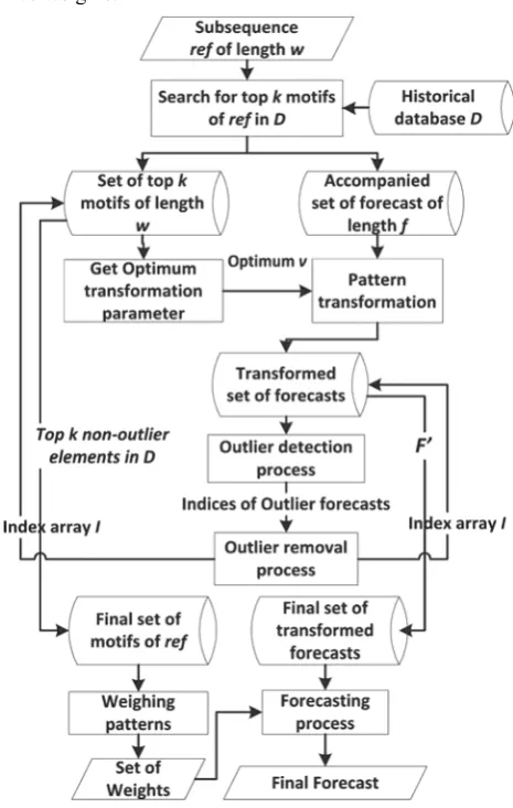
The proposed technique relies on the assumption that a temporal pattern will follow the behavior of its motifs from historical data. To implement this idea, we consider a reference temporal pattern ref that is the last subsequence of arbitrary length w in the investigated time series. Also, we consider the length of the required forecast subsequence of arbitrary length f. Then we go through six main steps: 1. Construct two time series database D and F drawn from

the available historical data. The database D consists of all subsequences of the same length as ref, each of which is subjected to measure its similarity to ref. The database F

consists of the subsequences - of length f each - that immediately follow the corresponding subsequences in D. 2. Search for the most similar patterns (motifs) of the

reference pattern ref inside the historical data D.

3. Transform the discovered motifs to bring them into the same numerical scale as ref using optimization techniques as described later in Algorithm 3. The transformation is hence applied to the forecast subsequence associated with the discovered motif.

4. Remove outliers from the set of the transformed forecast values. We used a simple outlier removal algorithm that is interquartile range.

ref gives a higher weight to its subsequent forecast values while keeping the sum of all weights=1. Equation (4) in Algorithm 5 describes the weighing method.

6. Calculate the final forecast by multiplying the forecast values following the discovered patterns by their respec-tive weights.

As shown in Fig. 2, the proposed algorithm utilizes the spirit of demand forecast algorithm in [1] to achieve our forecast goal, but we introduced two novel enhancements: 1. Systematic search for patterns similar to ref in historical

data using the speeded up brute force exact motif discoveryalgorithm in [5]. This algorithm simply searches for the k nearest neighbors of ref in D. The degree of similarity between subsequences in this process is measured using the Euclidean distance between the z-normalized time series to eliminate the effect of different numeric scales. It is described by [8]:

, ∑ (1)

where , are the z-normalization of

the time series , , . . , and , , . . ,

respectively, μ and σ are the mean and the standard deviation of each time series. The speeded up brute force exact motif discovery algorithm is a part of exact motif discovery in a time series which is an unsupervised learning task [6]. But due to the nature of our problem we are guiding the algorithm to search for the motifs of a particular pattern ref inside the historical database D.

2. Removing outliers from the proposed forecasts. Since our algorithm may produce a relatively big number of motifs of ref and hence some of these motifs may have extreme behavior in the points that follow the motif part. We employ an outlier removal algorithm to exclude these ex-treme points before weighing the remaining points to get our final forecast. 

Pseudo Code

Given: (1) The time series S, (2) Its last subsequence ref of arbitrary length w and (3) The History time series database of the same (or related) drug in other clinics. (4) The arbi-trary number of forecast points ahead f and (5) The arbitrary number of motifs to be discovered k.

Algorithm 1 : Main Algorithm Inputs: S, History, w, f,k

Output: A subsequence , . . , of length f that contains the forecast values of the original time series S.

1. ← , , … ,  

// set ref as the last subsequence in S with length w.

2. ← ∪

//Add the rest of S , … , as a new entry in History database.

3. ← 1

//Increase the number of time series in History by 1 4. ← 0 // A counter for the number of subsequences

in D, F databases.

5. ← 1

//Loop through every time series in History database.

6. ← 1

//Split each time series in History into sub-sequences of length w kept in D and the succeeding subsequence of length f kept into F.

7. ← , 1, … , 1

8. ← , … . . , 1

9. ← 1

10. END 11. END

12. Call Motif Discovery algorithm with D, ref, k.

13. Call Pattern Transformation algorithm for each of the top k motifs

14. Call Outlier Detection/Removal algorithm

15.Call patterns weighing and final forecast byD, ref ,F, I. The main algorithm splits the time series S of length n

into a last subsequence ref of arbitrary length w and first subsequence of length n-w. The first subsequence is added to the given History database of the drug consumption in other clinics to search for similar patterns of ref inside them. The algorithm exploits the database History to construct two databases D and F as in steps 7, 8. The D database contains every subsequence of length w as a candidate motif for ref. The F database contains the subsequences of length f that immediately follow the corresponding subsequence in D as a candidate forecast for S if its corresponding subsequence in D is chosen to be a motif for ref. Formally if

, 1, … , 1 then

, … , 1 .

To handle the probable seasonality in drug consumption data we can add an option when constructing the databases

D and F to consider only the subsequences in History that begins at the same calendar month that ref begins at. The purpose is not to consider drug consumption patterns in dif-ferent seasons as motifs. In this case, in step 6, the counter j

will begin at the required month and the loop step will be 12 to begin at the same month in every iteration.

Algorithm 2 : Motif Discovery

Inputs:  A database D of p time series. Each of which is of length = w.

 Ref,k.

Output: One dimensional array I of length k where

Ij is the location of the jthmotif for ref in D.

1. ← 1

2. ← ,

//Calculate the z-normalized Euclidean dis-tance between ref and Di

3. END

4. Find the set of smallest k values in array Dist. 5. Construct an ordering index array I for the indices of

Dist such that ∀ 1 1.

6. Return array I.

The Motif Discovery algorithm makes a one pass through the database D of all subsequences of interest. In step 2, it calculates the Euclidean distance between the z-normalized subsequence Di and the ref. The calculated distances are

kept in an array Dist. In step 4 we identify the smallest k

values in array Dist and then in step 5 we keep their indices in an array I. These indices of the smallest k values of Dist

are our target in the F subsequences database. The Euclid-ean distance in step 2 is applied upon the z-normalized time series to eliminate the effect of different numeric scales between ref and the compared time series in D.

Algorithm 3 : Pattern Transformation

In this algorithm we transform each of the motifs of ref

into the numeric scale of ref through two steps: 1. Make a vertical shift to the motif by adding the

difference between the averages of ref and its motif to every point in the motif, i.e.

(2) where is the vertically shifted value, is the

original value and .

By doing this we make the motif has the same average as ref.

2. Apply vertical extension /compression upon the pat-tern obtained from the previous vertical shift using the following equation [1]

min (3)

where is the transformed value , is the original value (the output of step 1) and is the ratio by which the original pattern extends vertically (if

1) or is compressed (if 1). The value of is de-termined by numerical optimization. The optimum value of is the value that generates the minimum MSE between the transformed motif and ref.

The aim of applying the pattern transformation in algo-rithm 3 upon each of the motifs of ref is to get its vertical displacement and optimum value for the parameter that makes its MSE distance from ref in its lowest possible value. Next we apply equations (2) and (3) with the same parameters , upon the F subsequence accompanied with each motif to obtain its transformed forecast. This trans-formation is adopted from [1] except that we use the Nelder-Mead non-linear optimization algorithm to obtain the opti-mum value for the parameter . Nelder-Mead algorithm is a direct search (derivative-free) algorithm that turns simplex search into an optimization algorithm efficiently [14].

Algorithm 4 : Outlier Detection/Removal algorithm Input:  The transformed time series database of

k time series of length f points each.

k, Index array

Output:  The time series database that carries the non-outlier forecast values of after removing outliers from each of its columns independently.

 Modified Index array I

1. ← 1

2. Get the first and third quartiles ( , respectively) of the array of the point ahead of the

trans-formed forecast where , ∀1 .

3. ← 0, ← 0 //initialize counters 4.

5. ← 1

6. IF lies in the range 1.5 ,

1.5 AND 0THEN

7. ← 1

8. ← //Build the non-outlier database

9. ← //Modify the Index I at point j

10. END IF 11. LOOP 12. END

13. RETURN , modified index array I for each point ahead j.

The set of transformed forecasts F are subjected to outlier detection and removal process for each point ahead of fore-cast independently. We used the interquartile range outlier removal algorithm in which we assume that Q1, Q3 are the lower and upper quartiles of the set of k forecast values respectively. Any forecast value out of the range

1.5 , 1.5 is considered as an

outlier. Also any negative value of the transformed F is removed as it could not be a drug consumption value.

Algorithm 5 : Patterns Weighing and Final Forecast Inputs:  The non-Outlier forecast database .

 The corresponding top k motifs of ref in the database D.

 The corresponding subsequences in the database Dist for the top k motifs.

 The ordering index I

1. ← 1

2. ← 0

//Initial value of the point ahead of forecast

3. ← 1

← 1

1 1

//Assign a weight to each pattern

//where ∑ at point j

(4) 4.

5. ←

//Use the weights and transformed forecasts to get final forecast

6. END 7. END

8. Return the subsequence , . . ,

Each of the resultant set of non-outlier forecasts at the jth point ahead of forecast , ∀ 1 , is a candidate to be our forecast goal. Instead of averaging them, we give each of them a weight that depends inversely on the Euclidean distance between its accompanied motif and ref

as in equation 4. The purpose is to give an advantage to the forecasts accompanied with the motifs most similar to ref. It can be easily proved that ∑ 1.

V. EXPERIMENTAL RESULTS

This section investigates the efficiency of the proposed algorithm against the efficiency of two other forecasting algorithms in terms of forecast accuracy. The dataset we have consists of 249 univariate time series each of which represents the consumption quantities of a certain drug in a certain family health unit (clinic) for a period of 60 consecu-tive months from July 2007 to June 2012. The forecast pro-cess is applied to each of the last 12 points in every time series. Each forecast is performed with every possible com-bination of the values of parameters w, k where w=5,6,…,12 and k=3,4,..,24. To measure the accuracy of our algorithm, the forecasted value is compared to the actual value by cal-culating the mean absolute percentage error MAPE [15]

where is the forecasted value and is the actual value and the sum runs over all the tested experiments assuming they are X experiments. The reason of choosing MAPE is that it is dimensionless and can represent a combination of forecasts of many different drugs having different consump-tion units and numeric scales. Also it can compare the performance of different forecasting methods. The lower the MAPE, the more accurate is a forecast [15].

The performance of our proposed algorithm is compared to other popular forecasting algorithms that are: 1- the expo-nential smoothing algorithm and 2- the average algorithm. If given a time series , … . , then the values of its expo-nential smoothing are , , . . , where 0,

, α 1 α , ∀ 2 [16]. Best results for the exponential smoothing algorithm are obtained experimentally in our dataset by setting 0.3. Regarding the average algorithm, its forecast for is ∑ .

Fig. 3 shows the effect of the length w of the ref pattern upon the performance of the proposed algorithm and the other two algorithms in terms of MAPE at the first point ahead of forecast. The performance of the proposed algorithm is presented with the continuous lines for three different values of parameter k (6, 9, and 24) to demonstrate the effect of small k values (6, 9) vs. the largest value 24. The Average and Exponential Smoothing algorithms are not affected by k since they depend only on ref and its length w. The proposed algorithm has lower MAPE (better perfor-mance) when increasing the values of w and k. For k≥6, the proposed algorithm is better than the other two algorithms for all values of w.

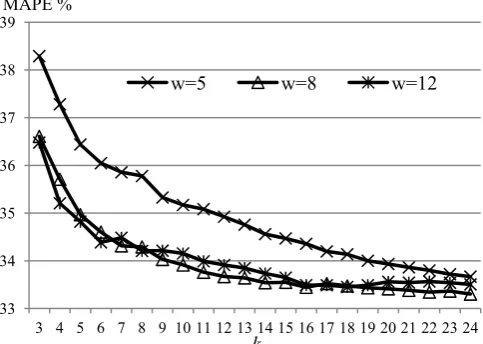
Regarding the effect of the parameter k upon the performance of the proposed algorithm, Fig. 4 shows the MAPE for the proposed algorithm vs. k where we tested 3≤

k≤ 24. We plotted three results having w=5, 8, 12. The results as expected shows poor performance at k=3 for all values of w and the performance is enhancing with increas-ing values of k. It is obvious that the enhancement is sharp for 3≤ k ≤ 8 and it becomes slow for 9≤ k ≤ 24 (approxi-mately no enhancement in this range for larger values of w). For small sample size between 3 and 8 (3≤ k ≤ 8) the outlier detection algorithm’s accuracy is relatively low and it does

1

(5)

Fig. 3: MAPE % for the proposed algorithm (continuous lines for k=6,9,24) , Average Algorithm, Exp. Smoothing Algorithm vs. parameter w values- at the first point ahead of forecast.

k=6 k=9

k=24

32 33 34 35 36 37 38

5 6 7 8 9 10 11 12

MAPE %

w

First point ahead Results

Average Algorithm-MAPE ExpSmoothing Algorithm MAPE

Fig. 4: MAPE % for the proposed algorithm vs. parameter k values. Three values for w parameters are plotted.

33 34 35 36 37 38 39

3 4 5 6 7 8 9 10 11 12 13 14 15 16 17 18 19 20 21 22 23 24 MAPE %

k

not capture many outlier forecasts which causes model inaccuracy. For larger set of forecasts (9≤k ≤ 24) the outlier detection algorithm can capture and remove outliers with higher accuracy. The turning point between small and large sample size depends on the used dataset and experimentally in our problem it is about 9. It is clear from Fig. 4 that no obvious performance enhancement by increasing the length of the ref pattern more than 8 points w≥8.

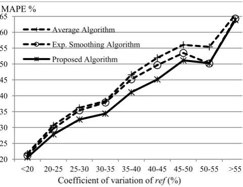
Fig. 5 illustrates the effect of the dispersion of the refer-ence pattern ref upon the performance of the proposed algorithm compared with the other two algorithms. The used dispersion measure is the coefficient of variation (CV) defined as the ratio of the standard deviation to the mean (for the ref pattern). It is a normalized measure of dispersion [17]. The figure shows that the proposed algorithm gives better performance than the other two algorithms for 25%

55%. The proposed algorithm gave the results in Fig. 5 by setting its parameters 8 (that gives the best results), and for all values of 5 12 to test all the available lengths of ref.

VI. CONCLUSIONANDFUTUREWORK The introduced algorithm is a multi-step ahead time series forecasting algorithm that represents an enhancement to the pattern matching for demand forecasting algorithm. We compensated a shortage in it by adding a systematic process for discovering patterns similar to the last pattern of arbitrary length of the time series. Our approach is using the motif discovery algorithm for getting the best matched patterns for the reference pattern. As a side effect of getting too much similar patterns, the forecast points corresponding to some of the discovered patterns may represent outliers. An outlier removal algorithm is merged before getting the final forecast to handle this issue. The new method out-performs the average and exponential smoothing algorithms when using nine or more motifs for the reference pattern. Also better performance is obtained with bigger values of the reference pattern’s length till its length reaches 8 points where the enhancements become slow. The proposed algorithm outperforms the other algorithms when the coefficient of variation of the pattern to be forecasted is between 25% and 55%. Future work includes extending experiments to other datasets and other fields like epidemics

forecasting from patients’ encounter data and from drug consumption patterns.

REFERENCES

[1] W. Yu, J. Graham and H. Min, "Dynamic Pattern Matching Using Temporal Data Mining for Demand Forecasting”, in Proc. of International Conference of Electronic Business, Taiwan, pp. 400-402,Dec. 2002.

[2] L. Aburto, and R. Weber, "Improved Supply Chain Management Based on Hybrid Demand Forecasts”, Journal of Applied Soft Computing, Vol. 7, Issue 1, Pages 136-144, 2007.

[3] W.C. Wang, K.W. Chau, C.T. Cheng, and L. Qiu ,"A Comparison of Performance of Several Artificial Intelligence Methods for Forecasting Monthly Discharge Time Series”, Journal of Hydrology

,Vol. 374, Issue 3-4, Pages 294-306,2009.

[4] N. K. Ahmed, A. F. Atiya, N. E. Gayar, and H. El-Shishiny, "An Empirical Comparison of Machine Learning Models for Time Series Forecasting”, Journal of Econometric Reviews, Vol. 29 , Issue 5 , Pages 594-621,2010.

[5] A. Mueen, E. Keogh, Q. Zhu, S. Cash, and B. Westover, "Exact Discovery of Time Series Motifs”, in Proc. of International Conference on Data Mining (SDM’09), USA, pp. 473-484, April 30 - May 2, 2009.

[6] N. Castro, and P. Azevedo,"Time Series Motifs Statistical Significance”, in Proc. of International Conference on Data Mining (SDM’11), USA, pp. 687-698, April 28-30, 2011.

[7] B. Chiu, E. Keogh, and S. Lonardi, “Probabilistic Discovery of Time Series Motifs”, in Proc. of 9th ACM SIGKDD International Conference on Knowledge Discovery and Data Mining (KDD’03), USA, pp. 493-498, August 24 - 27, 2003.

[8] A. Mueen, E. Keogh, and N. Bigdely-Shamlo, "Finding Time Series Motifs in Disk-Resident Data”, in Proc. of 9th IEEE International Conference on Data Mining,USA, pp. 367-376,Dec. 6-9, 2009. [9] N. Castro, and P. Azevedo, “Multiresolution Motif Discovery in Time

Series”, in Proc. of International Conference on Data Mining (SDM’10), USA, Vol. 21, pp. 665-676, April 29 - May 1, 2010. [10] A. R. Soroush, and N. Kamal-Abadi, "Review on Applications of

Artificial Neural Networks in Supply Chain Management and Its Future”, Journal of World Applied Sciences,Vol. 6, Pages 12-18,2009. [11] K. Bansal, S. Vadhavkar, and A. Gupta, "Brief Application

Description Neural Networks Based Forecasting Techniques for Inventory Control Applications”, Journal of Data Mining and Knowledge Discovery, Vol. 102 ,No. 1, Pages 97-102,1998.

[12] M. Khashei and M. Bijari, “A New Hybrid Methodology for Nonlinear Time Series Forecasting”, Modelling and Simulation in Engineering, Vol. 2011, Article ID 379121, Pages 1-5, 2011. [13] J. Lin, E. Keogh, S. Lonardi, and P. Patel, "Finding Motifs in Time

Series”, in Proc. of 2nd Workshop on Temporal Data Mining, at the 8th ACM (SIGKDD) International Conference on Knowledge Discovery and Data Mining, Canada , pp. 53 - 68, 23-26 July ,2002. [14] R. Lewis, V. Torczon, M. Trosset, "Direct Search Methods: Then and

Now". Journal of Computational and Applied Mathematics, Vol.124, Issue: 1-2, Pages 191-207, 2000.

[15] I. Klevecka, "Short-Term Traffic Forecasting with Neural Networks".

Journal of Transport and Telecommunication, Vol.12, No 2, Pages 20-27, 2011.

[16] E.Ostertagova and O. Ostertag. "The Simple Exponential Smoothing Model". in Proc. of 4th International Conference on Modelling of Mechanical and Mechatronic Systems, Slovak Republic, pp.380-384,Sep. 20-22, 2011.

[17] Y.Zhang, S.Hyon Baik, A.Fendrick, and K.Baicker, "Comparing Local and Regional Variation in Health Care Spending". New England Journal of Medicine, Vol. 376, pages: 1724-1731, 2012. Fig. 5: MAPE for the proposed algorithm, Average Algorithm, Exp.

Smoothing Algorithm against the coefficient of variation (CV) of ref. 20

25 30 35 40 45 50 55 60 65

<20 20-25 25-30 30-35 35-40 40-45 45-50 50-55 >55 MAPE %

Coefficient of variation of ref(%) Average Algorithm

Exp. Smoothing Algorithm