A Sketch Algorithm for Estimating Two Way and Multi Way Associations

and Multi-Way Associations

Ping Li

Stanford University

Kenneth W. Church

We should not have to look at the entire corpus (e.g., the Web) to know if two (or more) words are strongly associated or not. One can often obtain estimates of associations from a small sample. We develop a sketch-based algorithm that constructs a contingency table for a sample. One can estimate the contingency table for the entire population using straightforward scaling. However, one can do better by taking advantage of the margins (also known as document frequencies). The proposed method cuts the errors roughly in half over Broder’s sketches.

1. Introduction

We develop an algorithm for efficiently computing associations, for example, word associations.1_{Word associations (co-occurrences, or joint frequencies) have a wide range} of applications including: speech recognition, optical character recognition, and infor-mation retrieval (IR) (Salton 1989; Church and Hanks 1991; Dunning 1993; Baeza-Yates and Ribeiro-Neto 1999; Manning and Schutze 1999). TheKnow-It-Allproject computes such associations at Web scale (Etzioni et al. 2004). It is easy to compute a few association scores for a small corpus, but more challenging to compute lots of scores for lots of data (e.g., the Web), with billions of Web pages (D) and millions of word types.

Web search engines produce estimates of page hits, as illustrated in Tables 1– 3.2 Table 1 shows hits for two high frequency words,a and the, suggesting that the total number of English documents is roughlyD≈1010. In addition to the two high-frequency words, there are three low-high-frequency words selected from The New Oxford Dictionary of English (Pearsall 1998). The low-frequency words demonstrate that there are many hits, even for relatively rare words.

How many page hits do “ordinary” words have? To address this question, we ran-domly picked 15 pages from a learners’ dictionary (Hornby 1989), and selected the first en-try on each page. According to Google, there are 10 million pages/word (median value, aggregated over the 15 words). To compute all two-way associations for the 57,100 en-tries in this dictionary would probably be infeasible, let alone all multi-way associations.

∗Department of Statistical Science, Cornell University, Ithaca, NY 14853. E-mail: [email protected]. ∗∗Microsoft Research, Microsoft Corp., Redmond, WA 98052. E-mail: [email protected].

1 This paper considers boolean (0/1) data. See Li, Church, and Hastie (2006, 2007) for generalizations to real-valued data (andl_pdistances).

2 All experiments with MSN.com and Google were conducted in August 2005.

Table 1

Page hits for a few high-frequency words and a few low-frequency words (as of August 2005).

Query Hits (MSN.com) Hits (Google)

A 2,452,759,266 3,160,000,000

The 2,304,929,841 3,360,000,000

Kalevala 159,937 214,000

Griseofulvin 105,326 149,000

Saccade 38,202 147,000

Table 2

Estimates of page hits are not always consistent. Joint frequencies ought to decrease

monotonically as we add terms to the query, but estimates produced by current state-of-the-art search engines sometimes violate this invariant.

Query Hits (MSN.com) Hits (Google)

America 150,731,182 393,000,000

America, China 15,240,116 66,000,000

America, China, Britain 235,111 6,090,000 America, China, Britain, Japan 154,444 23,300,000

Table 3

This table illustrates the usefulness of joint counts in query planning for databases. To minimize intermediate writes, the optimal order of joins is: ((“Schwarzenegger”∩“Austria”)∩

“Terminator”)∩“Governor,” with 136,000 intermediate results. The standard practice starts with the least frequent terms, namely, ((“Schwarzenegger”∩“Terminator”)∩“Governor”)∩ “Austria,” with 579,100 intermediate results.

Query Hits (Google)

Austria 88,200,000

Governor 37,300,000

One-way Schwarzenegger 4,030,000

Terminator 3,480,000

Governor, Schwarzenegger 1,220,000

Governor, Austria 708,000

Schwarzenegger, Terminator 504,000

Two-way Terminator, Austria 171,000

Governor, Terminator 132,000

Schwarzenegger, Austria 120,000

Governor, Schwarzenegger, Terminator 75,100 Three-way Governor, Schwarzenegger, Austria 46,100 Schwarzenegger, Terminator, Austria 16,000

Governor, Terminator, Austria 11,500

Four-way Governor, Schwarzenegger, Terminator, Austria 6,930

Sampling can make it possible to work in physical memory, avoiding disk accesses. Brin and Page (1998) reported an inverted index of 37.2 GBs for 24 million pages. By extrapolation, we should expect the size of the inverted indexes for current Web scale to be 1.5 TBs/billion pages, probably too large for physical memory. A sample is more manageable.

When estimating associations, it is desirable that the estimates be consistent. Joint frequencies ought to decrease monotonically as we add terms to the query. Table 2 shows that estimates produced by current search engines are not always consistent.

1.1 The Data Matrix, Postings, and Contingency Tables

We assume a term-by-document matrix,A, withn rows (words) and Dcolumns (doc-uments). Because we consider boolean (0/1) data, the (i,j)th entry of Ais 1 if wordi occurs in document jand 0 otherwise. Computing all pair-wise associations ofAis a matrix multiplication,AAT_.

Because word distributions have long tails, the term-by-document matrix is highly sparse. It is common practice to avoid materializing the zeros inA, by storing the matrix in adjacency format, also known aspostings, and an inverted index (Witten, Moffat, and Bell 1999, Section 3.2). For each word W, the postings list, P, contains a sorted list of document IDs, one for each document containing W.

Figure 1(a) shows a contingency table. The contingency table for words W1and W2 can be expressed as intersections (and complements) of their postings P1and P2in the obvious way:

a=|P1∩P2|, b=|P1∩ ¬P2|, c=|¬P1∩P2|, d=|¬P1∩ ¬P2| (1)

where¬P1 is short-hand forΩ−P1, andΩ ={1, 2, 3,. . .,D}is the set of all document IDs. As shown in Figure 1(a), we denote the margins byf1=a+b=|P1|andf2=a+ c=|P2|.

For larger corpora, it is natural to introduce sampling. For example, we can ran-domly sample Ds (out of D) documents, as illustrated in Figure 1(b). This sampling

scheme, which we callsampling over documents, is simple and easy to describe—but we can do better, as we will see in the next subsection.

Figure 1

(a) A contingency table for word W1and word W2. Cellais the number of documents that contain both W1and W2,bis the number that contain W1but not W2,cis the number that contain W2but not W1, anddis the number that contain neither. The margins,f1=a+band

1.2 Sampling Over Documents and Sampling Over Postings

Sampling over documents selectsDsdocuments randomly from a collection ofD

docu-ments, as illustrated in Figure 1.

The task of computing associations is broken down into three subtasks:

1. Compute sample contingency table.

2. Estimate contingency table for population from sample.

3. Summarize contingency table to produce desired measure of association: cosine, resemblance, mutual information, correlation, and so on.

Sampling over documents is simple and well understood. The estimation task is straightforward if we ignore the margins. That is, we simply scale up the sample in the obvious way: ˆaMF =asDDs. We refer to these estimates as the “margin-free” baseline.

However, we can do better when we know the margins,f1=a+bandf2=a+c(called document frequenciesin IR), using a maximum likelihood estimator (MLE) with fixed margin constraints.

Rare words can be a challenge for sampling over documents. In terms of the term-by-document matrix A, sampling over documents randomly picks a fraction (Ds

D) of

columns from A. This is a serious drawback because A is highly sparse (as word distributions have long tails) with a few high-frequency words and many low-frequency words. The jointly non-zero entries inAare unlikely to be sampled unless the sampling rateDs

D is high. Moreover, the word sparsity differs drastically from one word to another;

it is thus desirable to have a sampling mechanism that can adapt to the data sparsity with flexible sample sizes. One size does not fit all.

“Sampling over postings” is an interesting alternative to sampling over docu-ments. Unfortunately, it doesn’t work out all that well either (at least using a sim-ple straightforward imsim-plementation), but we present it here nevertheless, because it provides a convenient segue between sampling over documents and our sketch-based recommendation.

“Naive sampling over postings” obtains a random sample of sizek1 from P1, de-noted as Z1, and a random sample Z2of sizek2from P2. Also, we denoteaNs =|Z1∩Z2|. We then useaN

s to infera. For simplicity, assumek1=k2=kandf1=f2=f. It follows that3 _EaN

s

a

=k2

f2. In other words, under naive sampling over postings, one could

estimate the associations by f_k22aNs.

3 Suppose there aremdefectives amongNobjects. We randomly pickkobjects (without replacement) and obtainxdefectives. Thenxfollows a hypergeometric distribution,x∼HG(N,m,k). It is known that E(x)=

m

Nk. In our setting, suppose we know that among Z1(of sizek1), there areaZ1s samples that belong to the

original intersection P1∩P2. Similarly, suppose we know that there areaZ2s samples among Z2(of sizek2) that belong to P1∩P2. ThenaNs =|Z1∩Z2| ∼HG(a,aZ1s ,aZ2s ). Therefore E

aN_s=1

aaZ1s aZ2s . BecauseaZ1s

andaZ2_s are both random, we should use conditional expectations: EaN

s =E E aN

s|aZ1s ,aZ2s

=

E1

aaZ1s aZ2s

=1

aE

aZ1s

EaZ2s

. (Recall that Z1and Z2are independent.) Note thataZ1s ∼HG(f1,a,k1) andaZ2_s ∼HG(f₂,a,k₂), that is, E

aZ1_s = a

f1k1and E

aZ2_s = a

f2k2. Therefore, E

aN

s

=1

afa1k1

a f2k2, namely, E

aN_s

a

=k1k2

Figure 2

The proposed sketch method (solid curve) produces larger counts (as) with less work (k). With “naive sampling over postings,” there is an undesirable quadratic: EaNs

a

=k2

f2 (dashed curve), whereas with sketches, Eas

a

≈k

f. These results were generated by simulation, withf1=f2=f=0.2D,D=105anda= 0.22, 0.38, 0.65, 0.80, 0.85f. There is only one dashed curve across all values ofa. There are different (but indistinguishable) solid curves depending ona.

Of course, the quadratic relation, EaNs

a

= k_f22, is undesirable; 1% effort returns only

0.01% useful information. Ideally, to maximize the signal, we’d like to see large counts in a small sample, not small counts in a large sample. The crux isas, which tends to have

the smallest counts. We’d like as to be as large as possible, but we’d also like to do as

little work (k) as possible. The next subsection on sketches proposes an improvement, where 1% effort returns roughly 1% useful information, as illustrated in Figure 2.

1.3 An Improvement Based on Sketches

A sketch is simply the front of the postings (after a random permutation). We find it helpful, as an informal practical metaphor, to imagine a virtual machine architecture where sketches (Broder 1997), the front of the postings, reside in physical memory, and the rest of the postings are stored on disk. More formally, the sketch, K=MINk(π(P)),

contains theksmallest postings, after applying a random permutationπto document IDs,Ω ={1, 2, 3,. . .,D}, to eliminate whatever structure there might be.

Given two words, W1 and W2, we have two sets of postings, P1 and P2, and two sketches, K1=MINk1(π(P1)) and K2=MINk2(π(P2)). We construct a sample

contin-gency table from the two sketches. LetΩs={1, 2, 3,. . .,Ds}be the sample space, where

Dsis set to min(max(K1), max(K2)). With this choice ofDs, all the document IDs in the

sample space,Ωs, can be assigned to the appropriate cell in the sample contingency table

without looking outside the sketch. One could use a smaller Ds, but doing so would

throw out data points unnecessarily.

The sample contingency table is constructed from K1 and K2 inO(k1+k2) time, using a straightforward linear pass over the two sketches:

as=|K1∩K2∩Ωs|=|K1∩K2| bs=|K1∩ ¬K2∩Ωs|

The final step is an estimation task. The margin-free (MF) estimator recovers the original contingency table by a simple scaling. For better accuracy, one could take advantage of the margins by using a maximum likelihood estimator (MLE).

With “sampling over documents,” it is convenient to express the sampling rate in terms ofDsandD, whereas with sketches, it is convenient to express the sampling rate

in terms ofkandf. The following two approximations allow us to flip back and forth between the two views:

E

Ds

D

≈min

k1 f1,

k2 f2

(3)

E

D Ds

≈max

f1 k1,

f2 k2

(4)

In other words, using sketches with size k, the corresponding sample size Ds in

“sampling over documents” would beDs≈ D_fk, where D_f represents the data sparsity.

Because the estimation errors (variances) are inversely proportional to sample size, we know the proposed algorithm improves “sampling over documents” by a factor proportional to the data sparsity.

1.4 Improving Estimates Using Margins

When we know the margins, we ought to use them. The basic idea is to maximize the likelihood of the sample contingency table under margin constraints. In the pair-wise case, we will show that the resultant maximum likelihood estimator is the solution to a cubic equation, which has a remarkably accurate quadratic approximation.

The use of margins for estimating contingency tables was suggested in the 1940s (Deming and Stephan 1940; Stephan 1942) for a census application. They developed a straightforward iterative estimation method called iterative proportional scaling, which was an approximation to the maximum likelihood estimator.

Computing margins is usually much easier than computing interactions. For a data matrixAofnrows andDcolumns, computing all marginall2norms costs onlyO(nD), whereas computing all pair-wise associations (orl2distances) costsO(n2D). One could compute the margins in a separate prepass over the data, without increasing the time and space complexity, though we suggest computing the margins while applying the random permutationπto all the document IDs on all the postings.

1.5 An Example

Let’s start with conventional random sampling over documents, using a running exam-ple in Figure 3. We choose a samexam-ple ofDs=18 documents randomly out of a collection

of D=36. After applying the random permutation, document IDs will be uniformly random. Thus, we can construct the random sample by picking anyDsdocuments. For

convenience, we pick the firstDs. The sample contingency table is then constructed, as

illustrated in Figure 3.

The recommended procedure is illustrated in Figure 4. The two sketches, K1 and K2, are highlighted in the large box. We find it convenient, as an informal practi-cal metaphor, to think of the large box as physipracti-cal memory. Thus, the sketches re-side in physical memory, and the rest are paged out to disk. We choose Ds to be

contin-Figure 3

In this example, the corpus containsD=36 documents. The population is:Ω ={1, 2,. . .,D}. The sample space isΩs={1, 2,. . .,Ds}, whereDs=18. Circles denote documents containing W1, and squares denote documents containing W2. The sample contingency table is:as= |{4, 15}|=2,bs=|{3, 7, 9, 10, 18}|=5,cs=|{2, 5, 8}|=3,ds=|{1, 6, 11, 12, 13, 14, 16, 17}|=8.

Figure 4

This procedure, which we recommend, produces the same sample contingency table as in Figure 3:as=2,bs=5,cs=3, andds=8. The two sketches, K1and K2(larger shaded box), reside in physical memory, and the rest of the postings are paged out to disk. K1contains of the firstk1=7 document IDs in P1and K2contains of the firstk2=7 IDs in P2. We assume P1and P2are already permuted, otherwise we should writeπ(P1) andπ(P2) instead.

Ds=min(max(K1), max(K2))=min(18, 21)=18. The sample contingency table is computed from the sketches (large box) in timek1+k2, but documents exceedingDsare excluded fromΩs (small box), because we can’t tell if they are in the intersection or not, without looking outside the sketch. As it turns out, 19 is in the intersection and 21 is not.

gency table forΩ_s={1, 2, 3,. . .,Ds}in physical memory in timeO(k1+k2) from K1and K2. In this example, documents 19 and 21 (highlighted in the smaller box) are excluded fromΩs. It turns out that 19 is part of the intersection, and 21 is not, but we would have

to look outside the sketches (and suffer a page fault) to determine that. The resulting sample contingency table is the same as in Figure 3:

as =|{4, 15}|=2 bs=|K1∩Ωs| −as=7−2=5

cs=|K2∩Ωs| −as=5−2=3 ds=Ds−(as+bs+cs)=8

1.6 A Five-Word Example

Figure 5 shows an example with more than two words. There areD=15 documents in the collection. We generate a random permutationπas shown in Figure 5(b). For every ID in postings Piin Figure 5(a), we apply the random permutationπ, but we only store

thekismallest IDs as a sketch Ki, that is, Ki=MINki(π(Pi)). In this example, we choose

k1=4,k2 =4,k3=4,k4=3,k5 =6. The sketches are stored in Figure 5(c). In addition, becauseπ(Pi) operates on every ID in Pi, we know the total number of non-zeros in Pi,

denoted byfi=|Pi|.

Figure 5

The original postings sets are given in (a). There areD=15 documents in the collection. We generate a random permutationπas shown in (b). We applyπto the postings Piand store the sketch Ki=MINki(π(Pi)). For example,π(P1)={11, 13, 1, 12, 15, 6, 8}. We choosek1= 4; and

hence the four smallest IDs inπ(P1) are K1={1, 6, 8, 11}. We choosek2=4,k3=4,k4=3, andk5=6.

just two words in the vocabulary.) We calculate, from sketches K1 and K2, the sample inner product as,(1,2) =|{6}|=1, and the corresponding corpus sample size, denoted by Ds,(1,2) =min(max(K1), max(K2))=min(11, 12)=11. Therefore, the “margin-free” estimate ofa(1,2)is simplyas,(1,2)DsD,(1,2) =1

15 11=1.4.

This estimate can be compared to the “truth,” which is obtained from the complete postings list, as opposed to the sketch. In this case, P1 and P2 have 4 documents in common. And therefore, the estimation error is 4−1.4 or 2.6 documents.

Similarly, for P1 and P5, Ds,(1,5) =min(11, 6)=6, as,(1,5)=2. Hence, the “margin-free” estimate ofa(1,5)is simply 2156 =5.0. In this case, the estimate matches the “truth” perfectly.

The procedure can be easily extended to more than two rows. Suppose we would like to estimate the three-way inner product (three-way joins) among P1, P4, and P5, denoted by a(1,4,5). We calculate the three-way sample inner product from K1, K4, and K5, as,(1,4,5)=|{6}|=1, and the corpus sample size Ds,(1,4,5)= min(max(K1), max(K4), max(K5))=min(11, 12, 6)=6. Then the “margin-free” estimate ofa(1,4,5)is 1156 =2.5.

Of course, we can improve these estimates by taking advantage of the margins.

2. Applications

There is a large literature on sketching techniques (e.g., Alon, Matias, and Szegedy 1996; Broder 1997; Vempala 2004). Such techniques have applications in information retrieval, databases, and data mining (Broder et al. 1997; Haveliwala, Gionis, and Indyk 2000; Haveliwala et al. 2002).

Broder’s sketches (Broder 1997) were originally introduced to detect duplicate documents in Web crawls. Many URLs point to the same (or nearly the same) HTML blobs. Approximate answers are often good enough. We don’t need to find all such pairs, but it is handy to find many of them, without spending more than it is worth on computational resources.

Section 1 mentioned page hit estimation. If we have a two-word query, we’d like to know how many pages mention both words. We assume that pre-computing and storing page hits is infeasible, at least not for infrequent pairs of words (and multi-word sequences).

It is customary in information retrieval to start with a large boolean term-by-document matrix. The boolean values indicate the presence or absence of a term in a document. We assume that these matrices are too large to store in physical memory. Depending on the specific applications, we can construct an inverted index and store sketches either for terms (to estimate word association) or for documents (to estimate document similarity).

2.1 Association Rule Mining

“Market-basket” analysis and association rules (Agrawal, Imielinski, and Swami 1993; Agrawal and Srikant 1994; Agrawal et al. 1996; Hastie, Tibshirani, and Friedman 2001, Chapter 14.2) are useful tools for mining commercial databases. Commercial databases tend to be large and sparse (Aggarwal and Wolf 1999; Strehl and Ghosh 2000). Various sampling algorithms have been proposed (Toivonen 1996; Chen, Haas, and Scheuermann 2002). The proposed algorithm scales better than traditional ran-dom sampling (i.e., a fixed sample of columns of the data matrix) for reasons men-tioned earlier. In addition, the proposed algorithm makes it possible to estimate association rules on-line, which may have some advantage in certain applications (Hidber 1999).

2.2 All Pair-Wise Associations (Distances)

In many applications, including distance-based classification or clustering and bi-gram language modeling (Church and Hanks 1991), we need to compute all pair-wise asso-ciations (or distances). Given a data matrix Aof n rows and Dcolumns, brute force computation of AAT would cost O(n2_{D), or more efficiently, O(n}2_{f¯), where ¯f is the} average number of non-zeros among all rows of A. Brute force could be very time-consuming. In addition, when the data matrix is too large to fit in the physical memory, the computation may become especially inefficient.

Using our proposed algorithm, the cost of computing AAT _{can be reduced to} O(nf¯)+O(n2_{k), where ¯}¯ _{k is the average sketch size. It costs O(nf}¯_{) for constructing} sketches and O(n2_{k) for computing all pair-wise associations. The savings would be}¯ significant when ¯kf¯. Note thatAAT_{is called “Gram Matrix” in machine learning; and} various algorithms have been proposed for speeding up the computation (e.g., Drineas and Mahoney 2005).

Ravichandran, Pantel, and Hovy (2005) computed pair-wise word associations (boolean data) amongn≈0.6 million nouns inD≈70 million Web pages, using random projections. We have discovered that in boolean data, our method exhibits (much) smaller errors (variances); but we will present the detail in other papers (Li, Church, and Hastie 2006, 2007).

2.3 Database Query Optimization

In databases, an important task is to determine the order of joins, which has a large impact on the system performance (Garcia-Molina, Ullman, and Widom 2002, Chapter 16). Based on the estimates of two-way, three-way, and even higher-order join sizes, query optimizers construct a plan to minimize a cost function (e.g., intermediate writes). Efficiency is critical as we certainly do not want to spend more time optimizing the plan than executing it.

We use an example (calledGovernator) to illustrate that estimates of two-way and multi-way association can help the query optimizer.

Table 3 shows estimates of hits for four words and their two-way, three-way, and four-way combinations. Suppose the optimizer wants to construct a plan for the query: “Governor, Schwarzenegger, Terminator, Austria.” The standard solution starts with the least frequent terms: ((“Schwarzenegger”∩“Terminator”)∩“Governor”)∩“Austria.” That plan generates 579,100 intermediate writes after the first and second joins. An im-provement would be ((“Schwarzenegger”∩“Austria”)∩“Terminator”)∩“Governor,” reducing the 579,100 down to 136,000.

3. Outline of Two-Way Association Results

To approximate the associations between words W1and W2, we work with sketches K1 and K2. We first determineDs =min(max(K1), max(K2)) and then construct the sample contingency table onΩs={1, 2,. . .,Ds}. The contingency table for the entire document

collection,Ω ={1, 2,. . .,D}, is estimated using a maximum likelihood estimator (MLE):

ˆ

aMLE=argmax a

Pr(as,bs,cs,ds|Ds;a) (5)

Section 5 will show that ˆaMLEis the solution to a cubic equation:

f1−a+1−bs

f1−a+1

f2−a+1−cs

f2−a+1

D−f1−f2+a D−f1−f2+a−ds

a

a−as =1 (6)

Instead of solving a cubic equation, we recommend a convenient and accurate quadratic approximation:

ˆ aMLE,a=

f1(2as+cs)+f2(2as+bs)−

f1(2as+cs)−f2(2as+bs) 2

+4f1f2bscs

2 (2as+bs+cs) (7)

We will compare the proposed MLE to two baselines: the independence baseline, ˆ

aIND, and the margin-free baseline, ˆaMF:

ˆ aIND=

f1f2

D ˆaMF=asDDs (8)

The margin-free baseline has smaller errors than the independence baseline, but we can do even better if we know the margins, as is common in practice.

These results are demonstrated both empirically and theoretically. In our field, it is customary to end with a large empirical evaluation. But there are always lingering ques-tions. Do the results generalize to other collections with more documents or different documents? This paper attempts to put such questions to rest by deriving closed-form expressions for the variances.

Var (ˆaMLE)≈

E

D Ds

−1 1

a+f1−a1 + 1

f2−a+ 1

D−f1−f2+a

, (9)

≈ max

f1 k1,

f2 k2

−1 1

a+_f1−a1 +_f2−a1 +_D−f1−f1 ₂+a

. (10)

Var (ˆaMF)=

ED Ds

−1 1

a+_D−a1 ≈

maxf1 k1,

f2 k2

−1 1

a +_D−a1

. (11)

These formulas establish the superiority of the proposed method over the alterna-tives, not just for a particular data set, but more generally. These formulas will also be used to determine stopping rules. How many samples do we need? We will use such an argument to suggest that a sampling rate of 10−3 may be sufficient for certain Web applications.

The proposed method generalizes naturally to multi-way associations, as presented in Section 6. Section 7 describes Broder’s sketches, which were designed for estimating resemblance, a particular association statistic. It will be shown, both theoretically and empirically, that our proposed method reduces the mean square error (MSE) by about 50%. In other words, the proposed method achieves the same accuracy with about half the sample size (work).

4. Evaluation of Two-Way Associations

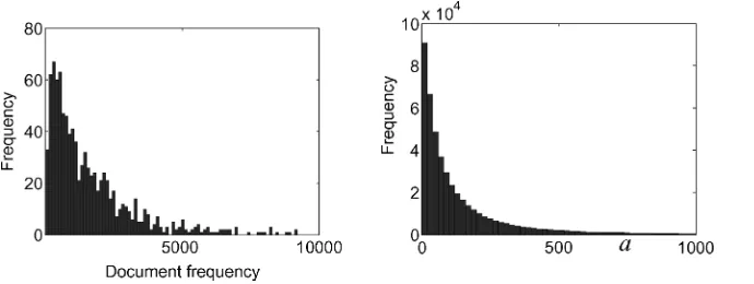
We evaluated our two-way association sampling/estimation algorithm with a chunk of Web crawls (D=216_{) produced by the crawler for MSN.com. We collected two sets} of English words which we will refer to as the small data set and the large data set. The small data set contains just four high frequency words: THIS,HAVE,HELP and PROGRAM (see Table 4), whereas the large data set contains 968 words (i.e., 468,028 pairs). The large data set was constructed by taking a random sample of English words that appeared in at least 20 documents in the collection. The histograms of the margins and co-occurrences have long tails, as expected (see Figure 6).

For the small data set, we applied 105 independent random permutations to the D=216 document IDs,Ω ={1, 2,. . .,D}. High-frequency words were selected so we could study a large range of sampling rates (k

f), from 0.002 to 0.95. A pair of sketches

Table 4

Small dataset: co-occurrences and margins for the population. The task is to estimate these values, which will be referred to as the gold standard, from a sample.

Case # Words Co-occurrence (a) Margin (f1) Margin (f2)

Case 2-1 THIS, HAVE 13,517 27,633 17,369

Case 2-2 THIS, HELP 7,221 27,633 10,791

Case 2-3 THIS, PROGRAM 3,682 27,633 5,327

Case 2-4 HAVE, HELP 5,781 17,369 10,791

Case 2-5 HAVE, PROGRAM 3,029 17,369 5,327

Case 2-6 HELP, PROGRAM 1,949 17,369 5,327

Monte Carlo trials. In this way, the small data set experiment made it possible to verify our theoretical results, including the approximations in the variance formulas.

The larger experiment contains many words with a large range of frequencies; and hence the experiment was repeated just six times (i.e., six different permutations). With such a large range of frequencies and sampling rates, there is a danger that some samples would be too small, especially for very rare words and very low sampling rates. A floor was imposed to make sure that every sample contains at least 20 documents.

4.1 Results from Large Monte Carlo Experiment

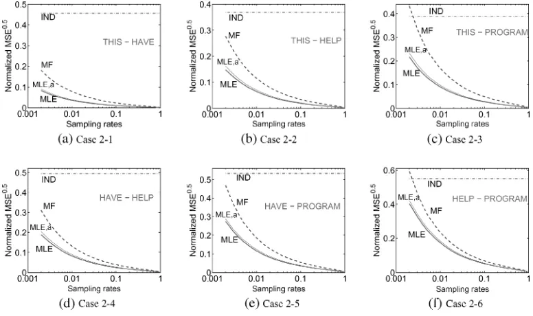
Figure 7 shows that the proposed methods (solid lines) are better than the baselines (dashed lines), in terms of MSE, estimated by the large Monte Carlo experiment over the small data set, as described herein. Note that errors generally decrease with sampling rate, as one would expect, at least for the methods that take advantage of the sample. The independence baseline (ˆaIND), which does not take advantage of the sample, has

very large errors. The sample is a very useful source of information; even a small sample is much better than no sample.

The recommended quadratic approximation, ˆaMLE,a, is remarkably close to the

ex-act MLE solution. Both of the proposed methods, ˆaMLE,a and ˆaMLE (solid lines), have

Figure 6

much smaller MSE than the margin-free baseline ˆaMF (dashed lines), especially at low

sampling rates. When we know the margins, we ought to use them.

Note that MSE can be decomposed into variance and bias:MSE(ˆa) = E (ˆa−a)2= Var (ˆa) +Bias2(ˆa). If ˆais unbiased,MSE(ˆa) = Var (ˆa) = SE2(ˆa), where SE is called “standard error.”

4.1.1 Margin Constraints Improve Smoothing.Though not a major emphasis of this paper, Figure 8 shows that smoothing is effective at low sampling rates, but only for those methods that take advantage of the margin constraints (solid lines as opposed to dashed lines). Figure 8 compares smoothed estimates (ˆaMLE, ˆaMLE,a, and ˆaMF) with their

un-smoothed counterparts. The y-axis reports percentage improvement of the MSE due to smoothing. Smoothing helps the proposed methods (solid lines) for all six word pairs, and hurts the baseline methods (dashed lines), for most of the six word pairs. We believe margin constraints keep the smoother from wandering too far astray; without margin constraints, smoothing can easily do more harm than good, especially when the smoother isn’t very good. In this experiment, we used the simple “add-one” smoother that replacesas,bs,cs, anddswithas+1,bs+1,cs+1, andds+1, respectively. We could

have used a more sophisticated smoother (e.g., Good–Turing), but if we had done so, it would have been harder to see how the margin constraints keep the smoother from wandering too far astray.

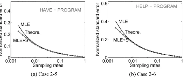
4.1.2 Monte Carlo Verification of Variance Formula. How accurate is the ap-proximation of the variance in Equations (9) and (11)? Figure 9 shows that the Monte Carlo simulation is remarkably close to the theoretical formula (9). Formula (11) is the same as (9), except that ED

Ds

is replaced with the approximation

Figure 7

The proposed estimator, ˆaMLE, outperforms the margin-free baseline, ˆaMF, in terms of

√

MSE

Figure 8

Smoothing improves the proposed MLE estimators but hurts the margin-free estimator in most cases. The vertical axis is the percentage of relative improvement in√MSE of each smoothed estimator with respect to its un-smoothed version.

Figure 9

Normalized standard error,SE(ˆaa), for the MLE. The theoretical variance formula (9) fits the simulation results so well that the curves are indistinguishable. Also, smoothing is effective in reducing variance, especially at low sampling rates.

max

f1 k1,

f2 k2

. Theoretically, we expect max

f1 k1,

f2 k2

≤E

D Ds

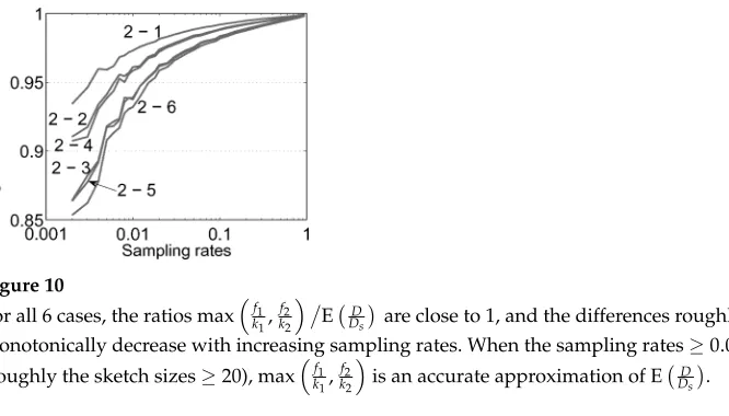
. Figure 10 verifies the inequality, and shows that the inequality is not too far from an equality. We will use (11) instead of (9), because the differences are not too large, and (11) is more convenient.

Figure 10

For all 6 cases, the ratios maxf1

k1,

f2

k2 E _D

Ds

are close to 1, and the differences roughly monotonically decrease with increasing sampling rates. When the sampling rates≥0.005 (roughly the sketch sizes≥20), maxf1

k1,

f2

k2

is an accurate approximation of ED Ds

.

Figure 11

Biases in terms of |E(ˆaa)−a|. ˆaMLEis practically unbiased. Smoothing increases bias slightly.

4.2 Results from Large Data Set Experiment

In Figure 12, the large data set experiment confirms the findings of the large Monte Carlo experiment: The proposed MLE method is better than the margin-free and inde-pendence baselines. The recommended quadratic approximation, ˆaMLE,a, is close to the

exact solution, ˆaMLE.

4.3 Rank Retrieval by Cosine

We are often interested in finding top ranking pairs according to some measure of sim-ilarity such as cosine. Performance improves with sampling rate for this task (as well as almost any other task; there is no data like more data), but nevertheless, Figure 13 shows that we can find many of the top ranking pairs, even at low sampling rates.

Note that the estimate of cosine, √a

f1f2, depends solely on the estimate ofa, because

Figure 12

(a) The proposed MLE methods (solid lines) have smaller errors than the baselines (dashed lines). We report the mean absolute errors (normalized by the mean co-occurrences, 188). All curves are averaged over six permutations. The two solid lines, the proposed MLE and the recommended quadratic approximation, are close to one another. Both are well below the margin-free (MF) baseline and the independence (IND) baseline. (b) Percentage of improvement due to smoothing. Smoothing helps MLE, but hurts MF.

Figure 13

We can find many of the most obvious associations with very little work. Two sets of cosine scores were computed for the 468,028 pairs in the large dataset experiment. The gold standard scores were computed over the entire dataset, whereas sample scores were computed over a sample of the data set. The plots show the percentage of agreement between these two lists, as a function ofS. As expected, agreement rates are high (≈100%) at high sampling rates (0.5). But it is reassuring that agreement rates remain pretty high (≈70%) even when we crank the sampling rate way down (0.003).

obtain if we used the entire data set. This section will compare the rankings based on a small sample to a gold standard, the rankings based on the entire data set.

(0.003). In other words, we can find many of the most obvious associations with very little work.

The same comparisons can be evaluated in terms of precision and recall, by fix-ing the top-LG gold standard list but varying the length of the sample list LS. More

precisely, recall=relevant/LG, and precision=relevant/LS, where “relevant” means

the retrieved pairs in the gold standard list. Figure 14 gives a graphical representation of this evaluation scheme, using notation in Manning and Schutze (1999), Chapter 8.1.

Figure 15 presents the precision–recall curves forLG=1%Land 10%L, whereL=

468, 028. For eachLG, there is one precision–recall curve corresponding to each sampling

rate. All curves indicate the precision–recall trade-off and that the only way to improve both precision and recall simultaneously is to increase the sampling rate.

4.4 Summary

To summarize the main results of the large and small data set experiments, we found that the proposed MLE (and the recommended quadratic approximation) have smaller

Figure 14

Definitions of recall and precision.L= total number of pairs.LG= number of pairs from the top of the gold standard similarity list.LS= number of pairs from the top of the reconstructed similarity list.

Figure 15

Precision–recall curves in retrieving the top 1% and top 10% gold standard pairs, at different sampling rates from 0.003 to 0.5. Note that the precision is always larger than LG

errors than the two baselines (the MF baseline and the independence (IND) base-line). Margin constraints improve smoothing, because the margin constraints keep the smoother from wandering too far astray. Monte Carlo simulations verified the variance formulas (9) and (11), and showed that the proposed MLE method is essentially un-biased. The ranking experiment showed that we can find many of the most obvious associations with very little work.

5. The Maximum Likelihood Estimator (MLE)

Section 4 evaluated the proposed method empirically; this section will explore the sta-tistical theory behind the method. The task is to estimate the contingency table (a,b,c,d) from the sample contingency table (as,bs,cs,ds), the margins, andD.

We can factor the (full) likelihood (probability mass function, PMF)Pr(as,bs,cs,ds;a) into

Pr(as,bs,cs,ds;a)=Pr(as,bs,cs,ds|Ds;a)×Pr(Ds;a) (12)

We seek theathat maximizes thepartial likelihoodPr(as,bs,cs,ds|Ds;a), that is,

ˆ

aMLE=argmax a

Pr(as,bs,cs,ds|Ds;a)=argmax a

logPr(as,bs,cs,ds|Ds;a) (13)

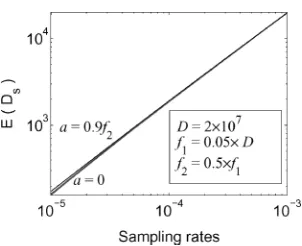
Pr(as,bs,cs,ds|Ds;a) is just the PMF of a two-way sample contingency table. That is relatively straightforward, butPr(Ds;a)is difficult. As illustrated in Figure 16, there is no strong dependency ofDsona, and therefore, we can focus on the easy part.

Before we delve into maximizingPr(as,bs,cs,ds|Ds;a) under margin constraints, we will first consider two simplifications, which lead to two baseline estimators. The inde-pendence baseline does not use any samples, whereas the margin-free baseline does not take advantage of the margins.

Figure 16

This experiment shows that E(Ds) is not sensitive toa.D=2×107_,f

5.1 The Independence Baseline

Independence assumptions are often made in databases (Garcia-Molina, Ullman, and Widom 2002, Chapter 16.4) and NLP (Manning and Schutze 1999, Chapter 13.3). When two words W1and W2are independent, the size of intersections,a, follows a hypergeo-metric distribution,

Pr(a)=

f1

a

D−f1 f2−a

D f2

, (14)

wheren m

= n!

m!(n−m)!. This distribution suggests an estimator

ˆ

aIND=E(a)= f1_Df2. (15)

Note that (14) is also a common null-hypothesis distribution in testing the indepen-dence of a two-way contingency table, that is, the so-called Fisher’s exact test (Agresti 2002, Section 3.5.1).

5.2 The Margin-Free Baseline

Conditional onDs, the sample contingency table (as,bs,cs,ds) follows themultivariate hypergeometricdistribution with moments4

E(as|Ds)= D_Dsa, E(bs|Ds)= D_Dsb, E(cs|Ds)= D_Dsc, E(ds|Ds)= D_Dsd,

Var(as|Ds)=Ds_Da

1− a

D

_D−D

s

D−1 (16)

where the term D−Ds

D−1 ≈1−

Ds

D, is known as the “finite population correction factor.”

An unbiased estimator and its variance would be

ˆ

aMF= _DD

sas, Var(ˆaMF|Ds)=

D2 D2

s

Var(as|Ds)=_DD s

1 1

a+_D−a1

D−Ds

D−1 . (17)

We refer to this estimator as “margin-free” because it does not take advantage of the margins.

The multivariate hypergeometric distribution can be simplified to a multinomial assuming “sample-with-replacement,” which is often a good approximation when Ds

D

is small. According to the multinomial model, an estimator and its variance would be:

ˆ

aMF,r= _DD

sas, Var(ˆaMF,r|Ds)=

D Ds

1 1

a +_D−a1

(18)

That is, for the margin-free model, the “sample-with-replacement” simplification still results in the same estimator but slightly overestimates the variance.

Note that these expectations in (16) hold both when the margins are known, as well as when they are not known, because the samples (as,bs,cs,ds) are obtained randomly

without consulting the margins. Of course, when we know the margins, we can do better than when we don’t.

5.3 The Exact MLE with Margin Constraints

Considering the margin constraints, the partial likelihood Pr(as,bs,cs,ds|Ds;a) can be

expressed as a function of a single unknown parameter,a:

Pr(as,bs,cs,ds|Ds;a)=

_a as _b bs _c cs _d ds _a+b+c+d

as+bs+cs+ds

=

_a

as

f1−a bs

_f 2−a

cs

_D−f1−f2+a ds

_D

Ds

∝ _(a−a!_a s)!×

(f1−a)! (f1−a−bs)!×

(f2−a)! (f2−a−cs)!×

(D−f1−f2+a)!

(D−f1−f2+a−ds)! (19)

= as−1

i=0

(a−i)×

bs−1

i=0

(f1−a−i)×

cs−1

i=0

(f2−a−i)×

ds−1

i=0

(D−f1−f2+a−i)

where the multiplicative terms not mentioning a are discarded, because they do not contribute to the MLE.

Let ˆaMLEbe the value ofathat maximizes the partial likelihood (19), or equivalently,

maximizes the log likelihood, logPr(as,bs,cs,ds|Ds;a):

as−1

i=0

log(a−i)+ bs−1

i=0

logf1−a−i

+ cs−1

i=0

logf2−a−i

+ ds−1

i=0

logD−f1−f2+a−i

whose first derivative, ∂logPr(as,bs,cs,ds|Ds;a)

∂a , is

as−1

i=0 1 a−i−

bs−1

i=0 1 f1−a−i−

cs−1

i=0 1 f2−a−i+

ds−1

i=0

1

D−f1−f2+a−i (20)

Because the second derivative, ∂2logPr(as,bs,cs,ds|Ds;a)

∂a2 ,

− as−1

i=0 1 (a−i)2 −

bs−1

i=0 1

(f1−a−i)2 −

cs−1

i=0 1

(f2−a−i)2 −

ds−1

i=0

1

(D−f1−f2+a−i)2

is negative, the log likelihood function is concave, and therefore, there is a unique maximum. One could solve (20) for ∂logPr(as,bs,cs,ds|Ds;a)

∂a =0 numerically, but it turns out

there is a more direct solution using the updating formula from (19):

Because we know that the MLE exists and is unique, it suffices to find theasuch that g(a)=1,

g(a)= _a−a_a s

f1−a+1−bs

f1−a+1

f2−a+1−cs

f2−a+1

D−f1−f2+a

D−f1−f2+a−ds =1 (21)

which is cubic ina(because the fourth term vanishes).

We recommend a straightforward numerical procedure for solvingg(a)=1. Note thatg(a)=1 is equivalent toq(a)=logg(a)=0. The first derivative ofq(a) is

q(a)=

1 f1−a+1−

1 f1−a+1−bs

+

1 f2−a+1−

1 f2−a+1−cs

(22)

+

1

D−f1−f2+a−

1

D−f1−f2+a−ds

+

1

a −a−1as

We can solve forq(a)=0 iteratively using Newton’s method:a(new)_=a(old)₋ q(a(old))

q(a(old)₎. See

Appendix 1 for a C code implementation.

5.4 The “Sample-with-Replacement” Simplification

Under the “sample-with-replacement” assumption, the likelihood function is slightly simpler:

Pr(as,bs,cs,ds|Ds;a,r)=

Ds

as,bs,cs,ds

a D

as_b

D bs_c

D cs_d

D ds

∝aas_(f

1−a)bs(f2−a)cs(D−f1−f2+a)ds (23)

Setting the first derivative of the log likelihood to be zero yields a cubic equation:

as

a −_f1b₋s _a−_f2c₋s _a+_D−f1d₋s _f2+a=0 (24)

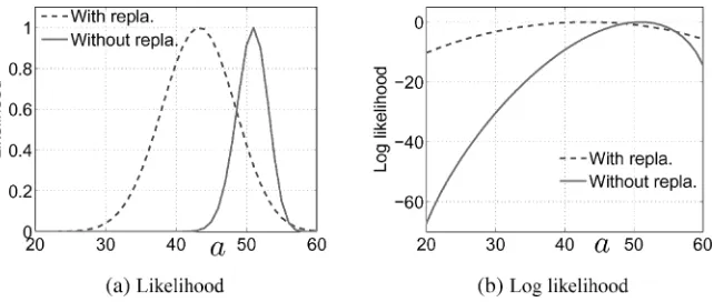
As shown in Section 5.2, using the margin-free model, the “sample-with-replacement” assumption amplifies the variance but does not change the estimation. With our proposed MLE, the “sample-with-replacement” assumption will change the estimation, although in general we do not expect the differences to be large. Figure 17 gives an (exaggerated) example, to show the concavity of the log likelihood and the difference caused by assuming “sample-with-replacement.”

5.5 A Convenient Practical Quadratic Approximation

Solving a cubic equation for the exact MLE may be so inconvenient that one may prefer the less accurate margin-free baseline because of its simplicity. This section derives a convenient closed-form quadratic approximation to the exact MLE.

The idea is to assume “sample-with-replacement” and that one can identifyasfrom

K1 without knowledge of K2. In other words, we assumeas(1)∼Binomial

as+bs,fa1

Figure 17

An example:as= 20,bs= 40,cs= 40,ds= 800,f1=f2= 100,D= 1000. The estimated ˆa= 43 for “sample-with-replacement,” and ˆa= 51 for “sample-without-replacement.” (a) The likelihood profile, normalized to have a maximum = 1. (b) The log likelihood profile, normalized to have a maximum = 0.

a(2)s ∼ Binomial

as+cs,fa2

, and as(1) and a(2)s are independent with a(1)s =as(2)=as.

The PMF ofa(1)s ,a(2)s

is a product of two binomials:

f1 as+bs

a f1

as_f

1−a f1

bs

×

f2 as+cs

a f2

as_f

2−a f2

cs

∝a2as_f

1−a bs

f2−a cs

(25)

Setting the first derivative of the logarithm of (25) to be zero, we obtain

2as

a −_f1b₋s _a−_f2c₋s _a=0 (26)

which is quadratic inaand has a convenient closed-form solution:

ˆ aMLE,a=

f1(2as+cs)+f2(2as+bs)−

(f1(2as+cs)−f2(2as+bs))2+4f1f2bscs

2 (2as+bs+cs) (27)

The second root can be ignored because it is always out of range:

f1(2as+cs)+f2(2as+bs)+

(f1(2as+cs)−f2(2as+bs))2+4f1f2bscs

2 (2as+bs+cs)

≥ f1(2as+cs)+f2(2as+bs)+|f1(2as+cs)−f2(2as+bs)|

2 (2as+bs+cs)

≥

f1 iff1(2as+cs)≥f2(2as+bs)

f2 iff1(2as+cs)<f2(2as+bs) ≥min(f1,f2)

5.6 The Conditional Variance and Bias

Usually, a maximum likelihood estimator is nearly unbiased. Furthermore, assuming “sample-with-replacement,” we can apply the large sample theory5 _{(Lehmann and} Casella 1998, Theorem 6.3.10), which says that ˆaMLE is asymptotically unbiased and

converges in distribution to a Normal with mean aand variance 1

I(a), where I(a), the expected Fisher Information, is

I(a)=−E

∂2

∂a2 logPr(as,bs,cs,ds|Ds;a,r)

=E

as

a2 + bs

(f1−a)2

+ cs

(f2−a)2

+ ds

(D−f1−f2+a)2 Ds

= E(as|Ds)

a2 +

E(bs|Ds)

f1−a

2 +E(cs|Ds)

f2−a

2 + E(ds|Ds)

D−f1−f2+a 2

= Ds

D

1

a+_f1−1 _a+_f21_−a+_D−f11_−f2+a

(28)

where we evaluate E(as|Ds), E(bs|Ds), E(cs|Ds), E(ds|Ds) by (16).

For “sampling-without-replacement,” we correct the asymptotic variance 1 I(a) by multiplying by the finite population correction factor 1−Ds

D:

Var (ˆaMLE|Ds)≈ _I(a)1

1−Ds

D

=

D Ds −1

1

a +_f11_−a+_f2−a1 +_D−f11_−f2+a

(29)

Comparing (17) with (29), we know that Var (ˆaMLE|Ds)<Var (ˆaMF|Ds), and the

dif-ference could be substantial. In other words, when we know the margins, we ought to use them.

5.7 The Unconditional Variance and Bias

Errors are a combination of variance and bias. Fortunately, we don’t need to be con-cerned about bias, at least asymptotically:

E (ˆaMLE−a)=E (E (ˆaMLE−a|Ds))→E(0)=0 (30)

The unconditional variance can be computed using the conditional variance formula:

Var (ˆaMLE)=E (Var (ˆaMLE|Ds))+Var (E (ˆaMLE|Ds))

→ E

D Ds

−1 1

a +_f1−a1 +_f2−a1 +_D−f1−f1 ₂+a

(31)

because E (ˆaMLE|Ds)→a, which is a constant. Hence Var (E (ˆaMLE|Ds))→0.

To evaluate ED Ds

exactly, we need PMFPr(Ds;a), which is unavailable. Even if it

were available, ED Ds

probably wouldn’t have a convenient closed-form.

Here we recommend the approximations, (3) and (4), mentioned previously. To de-rive these approximations, recall thatDs=min (max(K1), max(K2)). Using the discrete order statistics distribution (David 1981, Exercise 2.1.4),6_{we obtain:}

E (max(K1))= k1(D

+1) f1+1 ≈

k1

f1D, E (max(K2))≈ k2

f2D (32)

The min function can be considered to be concave. By Jensen’s inequality (see Cover and Thomas 1991, Theorem 2.6.2), we know that

E Ds D =E min

max(K1k1)

D ,

max(K2) D

≤min

E(max(K1)

D ,

E(max(K2) D

=min

k1 f1,

k2 f2

(33)

The reciprocal function is convex. Again by Jensen’s inequality, we have

E D Ds =E 1 Ds/D

≥ 1

EDs

D

≥max

f1 k1,

f2 k2

(34)

By replacing the inequalities with equalities, we obtain (35) and (36):

E Ds D ≈min k1 f1,

k2 f2 (35) E D Ds ≈max f1 k1,

f2 k2

(36)

In our experiments, when the sample size is reasonably large (Ds ≥20), the errors

in (35) and (36) are usually within 5%.

Approximations (35) and (36) provide an intuitive relationship between two views of the sampling rate: (a) Ds

D, which depends on corpus size and (b) kf, which depends on

the size of the postings. The difference between these two views is important when the term-by-document matrix is sparse, which is often the case in practice.

Using (36), we obtain the following approximation for the unconditional variance:

Var (ˆaMLE)≈

maxf1 k1,

f2 k2

−1 1

a+_f1−a1 +_f2−a1 +_D−f11_−f2+a

(37)

5.8 The Variance ofhhh(ˆaaaMLEMLEMLE)

We can estimate any functionh(a) byh(ˆaMLE). In practical applications,hcould be any

measure of association including cosine, resemblance, mutual information, etc. When h(a) is a nonlinear function ofa,h(ˆaMLE) will be biased. One can remove the bias to

some extent using Taylor expansions. See some examples in Li and Church (2005). Bias correction is important for small samples and highly nonlinear h’s (e.g., the log likelihood ratio, LLR).

The bias ofh(ˆaMLE) decreases with sample size. Precisely, thedelta method(Agresti

2002, Chapter 3.1.5) says that h(ˆaMLE) is asymptotically unbiased and the variance of

h(ˆaMLE) is

Var(h(ˆaMLE))→Var(ˆaMLE)(h(a))2 (38)

providedh(a) exists and is non-zero. Non-asymptotically, it is easy to show that

Var(h(ˆaMLE))≥Var(ˆaMLE)(h(a))2 ifh(a) is convex (39)

Var(h(ˆaMLE))≤Var(ˆaMLE)(h(a))2 ifh(a) is concave (40)

5.9 How Many Samples Are Sufficient?

The answer depends on the trade-off between computational costs (time and space) and estimation errors. For very infrequent words, we might afford to sample 100%. In general, a reasonable criterion is the coefficient of variation, cv = SE(ˆaa), SE=

Var(ˆa). We consider the estimate is accurate if the cv is below some thresholdρ₀(e.g.,ρ₀=0.1). The cv can be expressed as

cv=SE(ˆ_aa) ≈ 1_a

max

f1 k1,

f2 k2

−1 1

a+f1−a1 + 1

f2−a+ 1

D−f1−f2+a

(41)

Figure 18(a) plots the required sampling rate mink1 f1,

k2 f2

computed from (41). The

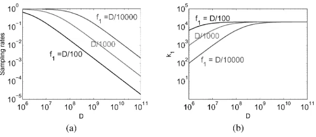
figure shows that at Web scale (i.e.,D≈10 billion), a sampling rate as low as 10−3may suffice for “ordinary” words (i.e., f1 ≈107=0.001D). Figure 18(b) plots the required sample sizek1, for the same experiment in Figure 18(a), where for simplicity, we assume

k1 f1 =

k2

f2. The figure shows that, afterDis large enough, the required sample size does

not increase as much.

To apply (41) to the real data, Table 5 presents the critical sampling rates and sample sizes for all pair-wise combinations of the four-word query Governor, Schwarzenegger, Terminator, Austria.Here we assume the estimates in Table 3 are exact. The table verifies that only a very small sample may suffice to achieve a reasonable cv.

5.10 Tail Bound and Multiple Comparisons Effect

Figure 18

(a) An analysis based on cv =SE

a = 0.1 suggests that we can get away with very low sampling rates. The three curves plot the critical value for the sampling rate, min

k1

f1,

k2

f2

, as a function of corpus size,D. At Web scale,D≈1010_{, sampling rates above 10}−2_{to 10}−4_{satisfy cv≤0.1, at} least for these settings off1,f2, anda. The settings were chosen to simulate “ordinary” words. The three curves correspond to three choices off1:D/100,D/1000, andD/10, 000.f2=f1/10,

a=f2/20. (b) The critical sample sizek1(assumingkf11 =

k2

f2), corresponding to the sampling rates in (a).

Table 5

The critical sampling rates and sample sizes (for cv = 0.1) are computed for all two-way combinations among the four wordsGovernor, Schwarzenegger, Terminator, Austria,assuming the estimated document frequencies and two-way associations in Table 3 are exact. The required sampling rates are all very small, verifying our claim that for “ordinary” words, a sampling rate as low as 10−3_{may suffice. In these computations, we usedD=5×10}9_{for the number of} English documents in the collection.

Query Critical Sampling Rate

Governor, Schwarzenegger 5.6×10−5

Governor, Terminator 7.2×10−4

Governor, Austria 1.4×10−4

Schwarzenegger, Terminator 1.5×10−4 Schwarzenegger, Austria 8.1×10−4

Terminator, Austria 5.5×10−4

we are estimating n(n−₂ 1) pairs simultaneously. A convenient approach is to bound the tail probability

Pr(|aˆMLE−a|> a)≤δ/p (42)

whereδ(e.g., 0.05) is the level of significance,is the specified accuracy (e.g., <0.5), andpis the correction factor for multiple comparisons. The most conservative choice is p= n2

2, known as the Bonferroni Correction. But often it is reasonable to letpbe much smaller (e.g.,p= 100).

Assuming ˆaMLE∼N(a, Var (ˆaMLE)), then, based on the known normal tail bound,

Pr(|aˆMLE−a|> a)≤2 exp

−_{2Var (ˆ}2a_a2 MLE)

=2 exp− 2 2cv2

(43)

combined with (42), leads to the following criterion on cv

cv≥

− 1

2 logδ/2p (44)

For example, if we letδ=0.05,p=100, and=0.4, then (44) will output cv≈0.1.

5.11 Sample Size Selection Based on Storage Constraints

Suppose we can compute the maximum allowed total samples, T, for example, based on the available memory. That is,n_i=1ki=T, wherenis the total number of words. We

could allocateTaccording to document frequenciesfj, that is,

kj=

fj

n i=1fi

T (45)

Usually, we will need to define a lower boundkland an upper boundku, which have

to be selected from engineering experience, depending on the specific applications. We will truncate the computed kj if it is outside [kl, ku]. Equation (45) implies a uniform

corpus sampling rate, which may not be always desirable, but the confinement by [kl, ku] can effectively vary the sampling rates.

More carefully, we can minimize the total number of “unused” samples. For a pair, Wiand Wj, if kfii ≥

kj

fj, then on average, there are

ki

fi −

kj

fj

fisamples unused in Ki. This

is the basic idea behind the following linear program for choosing the “optimal” sample sizes:

Minimize

n

i=1

n

j=i+1

fi

ki

fi −

kj

fj

+

+ fj

_k

j

fj −

ki

fi

+

subject to

n

i=1

ki=T, ki≤fi, kl≤ki≤ku (46)

where (z)+=max(0,z), is the positive part ofz. This program can be modified (possibly no longer a linear program) to consider other factors in different applications. For example, some applications may care more about the very rare words, so we would weight the rare words more.

5.12 When Will Sketches Not Perform Well?

In fact, it will do very well when both words are rare because the equivalent sampling rate Ds

D ≈min

k1 f1,

k2 f2

can be high, even 100%.

Whenf2f1, no sampling method can work well unless we are willing to sample P1 with a sufficiently large sample. Otherwise even if we let kf22 =100%, the corpus

sampling rate, Ds

D ≈

k1

f1, will be low. For example, Google estimates 14,000,000 hits

for Holmes, 37,500 hits for Diaconis, and 892 joint hits. Assuming D=5×109 and cv = 0.1, the critical sample size forHolmeswould have to be 1.4×106, probably too large as a sample.7

6. Extension to Multi-Way Associations

Many applications involve multi-way associations, for example, association rules, data-bases, and Web search. The “Governator” example in Table 3, for example, made use of both two-way and three-way associations. Fortunately, our sketch construction and estimation algorithm can be naturally extended to multi-way associations. We have already presented an example of estimating multi-way associations in Section 1.6. When we do not consider the margins, the estimation task is as simple as in the pair-wise case. When we do take advantage of margins, estimating multi-way associations amounts to a convex program. We will also analyze the theoretical variances.

6.1 Multi-Way Sketches

Suppose we are interested in the associations among m words, denoted by W1, W2, . . . , Wm. The document frequencies aref1,f2,. . ., andfm, which are also the lengths

of the postings P1, P2,. . ., Pm. There areN=2m combinations of associations, denoted

byx1,x2,. . .,xN. For example,

a=x1=|P1∩P2∩. . .∩Pm−1∩Pm|

x2=|P1∩P2∩. . .∩Pm−1∩ ¬Pm|

x3=|P1∩P2∩. . .∩ ¬Pm−1∩Pm|

. . .

xN−1=|¬P1∩ ¬P2∩. . .∩ ¬Pm−1∩Pm|

xN =|¬P1∩ ¬P2∩. . .∩ ¬Pm−1∩ ¬Pm| (47)

which can be directly corresponded to the binary representation of integers.

Using the vector and matrix notation, X=[x1,x2,. . .,xN]T, F=[f1,f2,. . .,fm,D]T,

where the superscript “T” stands for “transpose”, that is, we always work with col-umn vectors. We can write down the margin constraints in terms of a linear matrix equation as

AX=F (48)