Confidence estimation for translation prediction

Confidence Estimation for Translation Prediction

Simona Gandrabur

RALI, Universit´e de Montr´eal

[email protected]

George Foster

RALI, Universit´e de Montr´eal

[email protected]

Abstract

The purpose of this work is to investigate the use of machine learning approaches for confi-dence estimation within a statistical machine translation application. Specifically, we at-tempt to learn probabilities of correctness for various model predictions, based on the native probabilites (i.e. the probabilites given by the original model) and on features of the current context. Our experiments were conducted us-ing three original translation models and two types of neural nets (single-layer and multi-layer perceptrons) for the confidence estima-tion task.

1

Introduction

Most statistical models used in natural language appli-cations are capable in principle of generating probability estimates for their outputs. However, in practice, these estimates are often quite poor and are usually interpreted simply as scores that are monotonic with probabilities. There are many contexts where good estimates of true probabilities are desirable:

• in a decision-theoretic setting, posterior probabili-ties are required in order to choose the lowest-cost output for a given input.

• when a collection of different models is available for some problem, output probabilities provide a princi-pled and convenient way of combining them; and

• when multiplying conditional probabilities to com-pute joint distributions, the accuracy of the result is crucially dependent on the stability of the con-ditional estimates across different contexts—this is important for applications like speech recognition and machine translation that perform searches over

a large space of output sentences, represented as se-quences of words.

Given a statistical model that produces a probabilistic score, a straightforward way of obtaining a true probabil-ity is to use the score as input to another model whose output is interpreted as the desired probability. The idea is that the second model can learn how to transform the base model’s score by observing its performance on new text, possibly in conjunction with other features. This ap-proach, which is known as confidence estimation (CE), is widely used in speech recognition (Guillevic et al., 2002; Moreno et al., 2001; Sanchis et al., 2003; Stolcke et al., 1997) but is virtually unknown in other areas of natural language progessing (NLP).1

The alternatives to confidence estimation are tradi-tional smoothing techniques such as backing off to sim-pler models and cross validation, along with careful marginalization and scaling where applicable to obtain the desired posterior probabilities. There is some evi-dence (Wessel et al., 2001) that this approach can give results that are at least as good as those obtainable with an external CE model. However, CE as we present it here is not incompatible with traditional techniques, and has several practical advantages. First, it can easily incorpo-rate specialized features that are highly indicative of how well the base model will perform on a given input, but that may be of little use for the task of choosing the out-put. Since such features may be inconvenient to include in the base model, CE represents a kind of modulariza-tion, particularly as it may be possible to reuse some fea-tures for many different problems. Another advantage is that a CE layer is usually much smaller and easier to train than the baseline model; this means that it can be used to rapidly adapt a system’s performance to new domains. Finally, CE typically concentrates on only the top few

hy-1

potheses output by the baseline model, which is an easier task than estimating a complete distribution. This is es-pecially true when the hypotheses of interest are drawn from a joint distribution that may be impossible in prac-tice to enumerate.

In this paper we describe an application of confidence estimation to an interactive target-text prediction task in a translation setting, using two different types of neural nets: single-layer perceptron (SLPs) and multi-layer per-ceptrons (MLPs) with 20 hidden units.

The main issues that we investigate here are:

• the benefit that can be gained by using confidence estimates, in discrimination power and/or over-all application quality as computed by a simulation that estimates the benefit to the user;

• the use of different machine learning (ML) tech-niques for CE;

• the relevance of various confidence features; and

• model combinations: we experiment with various model combination schemes based on the CE layer in order to improve the over-all prediction accuracy of the application.

Among the more interesting results we will present are the comparisons between the discrimination capacity of the native probabilities and the probabilities of correct-ness produced by the CE layer. Depending on the un-derlying SMT model, we obtained a relative improve-ment in correct rejection rate (CR) ranging from3.90% to33.09% at a fixed0.80correct acceptance rate (CA) for prediction lengths of up to four words. We also mea-sured relative improvements of approximately 10% in es-timated benefit to the user with our application.

In the following section we briefly describe the text prediction application we are aiming to improve. Next we outline the CE approach and the evaluation methods we applied. Finally, we report the results obtained in our ex-periments and conclude with suggestions for future work.

2

Text Prediction for Translators

The application we are concerned with in this paper is an interactive text prediction tool for translators. The sys-tem observes a translator in the process of typing a target text and, after every character typed, has the opportunity to display a suggestion about what will come next, based on the source sentence under translation and the prefix of its translation that has already been typed. The transla-tor may incorporate suggestions into the text if they are helpful, or simply ignore them and keep typing.

Suggestions may range in length from 0 characters to the end of the target sentence; it is up to the system to

decide how much text to predict in a given context, bal-ancing the greater potential benefit of longer predictions against a greater likelihood of being wrong, and a higher cost to the user (in terms of distraction and editing) if they are wrong or only partially right.

Our solution to the problem of how much text to pre-dict is based on a decision-theoretic framework in which we attempt to find the prediction that maximizes the ex-pected benefit to the translator in the current context (Fos-ter et al., 2002b). Formally, we seek:

ˆx= argmax

x B(x|h,s), (1)

where x is a prediction about what will follow h in the translation of a source sentence s, and B(x|h,s) is the expected benefit in terms of typing time saved. As described in (Foster et al., 2002b), B(ˆx_m|h,s) =

P_l

k=0p(k|x,h,s)B(x|h,s, k) depends on two main

quantities: the probability p(k|x,h,s) that exactly k characters from the beginning of x are correct, and the benefit B(x|h,s, k) to the translator if this is the case. B(x|h,s, k) is estimated from a model of user behaviour—based on data collected in user trials of the tool—that captures the cost of reading a prediction and performing any necessary editing, as well as the some-what random nature of people’s decisions to accept. Pre-diction probabilitiesp(k|x,h,s)are derived from a statis-tical translation model forp(w|h,s), the probability that some wordwwill follow the target texthin the transla-tion of a source sentences.

Because optimizing (1) directly is expensive, we use a heuristic search procedure to approximateˆx. For each length m from 1 to a fixed maximum of M (4 in this paper), we perform a Viterbi-like beam search with the translation model to find the sequence of wordswˆ_m = w1, . . . , wmmost likely to follow h. For each such se-quence, we form a corresponding character sequenceˆx_m and evaluate its benefitB(ˆx_m,h,s). The final output is the predictionˆx_m with maximum benefit, or nothing if all benefit estimates are negative.

To evaluate the system, we simulate a translator’s ac-tions on a given source text, using an existing transla-tion as the text the translator wishes to type, and the user model to determine his or her responses to predictions and to estimate the resulting benefit. Further details are given in (Foster et al., 2002b).

2.1 Translation Models

We experimented with three different translation models forp(w|h,s). All have the property of being fast enough to support real-time searches for predictions of up to 5 words.

maximum entropy translation component that is an ana-log of the IBM translation model 2 (Brown et al., 1993). This model is described in (Foster, 2000). Its major weak-ness is that it does not keep track of which words in the current source sentence have already been translated, and hence it is prone to repeating previous suggestions. The second model, called Maxent2 below, is similar to Max-ent1 but with the addition of extra parameters to limit this behaviour (Foster et al., 2002a).

The final model, called Bayes below, is also described in (Foster et al., 2002a). It is a noisy-channel combination of a trigram language model and an IBM model 2 for the source text given target text. This model has roughly the same theoretical predictive capability as Maxent2, but un-like the Maxent models it is not discriminatively trained, and hence its native probability estimates tend to be much worse than theirs.

2.2 Computing Smoothed Conditional Probabilities

In order to calculate the character-based probabili-ties p(k|x,h,s) required for estimating expected ben-efit, we need to know the conditional probabilities p(w|w1, . . . , wi−1,h,s) that some word w will follow

w1, . . . , wi−1 in the context (h,s). These are derived

from correctness estimates obtained from our confidence-estimation layer as follows. As explained below, es-timates from the CE layer are in the form p(C = 1|wˆm,h,s), wherewˆ_mis the most probable prediction of length m according to the base translation model. Define a smoothed joint distribution over predictions of lengthmas:

ps(wm|h,s) =

½

p(C= 1|wˆm,h,s), wm=wˆm

p(wm|h,s)/zm, else

(2) wherep(w_m|h,s) = Qm_i=1p(w_i|w₁, . . . , w_i−1,h,s)is calculated from the conditional probabilities given by the base model; and

zm=₁₋1_p−_(Cp_{= 1}(wˆm_|wˆ|h,s) m,h,s)

is a normalization factor. Then the required smoothed conditional probabilities are estimated from the smoothed joint distributions in a straightforward way:

ps(w|w1, . . . , wi−1,h,s) = ps_p(w1, . . . , wi−1, w|h,s)

s(w1, . . . , wi−1|h,s) ,

wherep(w₁, . . . , w_i−1|h,s)≡1wheni= 1.

3

Confidence Estimation with Neural Nets

Our approach for CE consists in training neural nets to es-timate the conditional probability of correctnessp(C = 1|wˆm,h,s,{wm1, . . . ,wmn}), wherewˆm = w1m is the

most probable prediction of lengthmfrom an-best set of alternative predictions according to the base model. In our experiments the prediction lengthmvaries between 1 and4 andn is at most 5. As the n-best predictions {w1

m, . . . ,wnm}are themselves a function of the context,

we will simply note the conditional probability of cor-rectness byp(C= 1|wˆ_m,h,s).

We experimented with two types of neural nets: single-layer perceptrons (SLPs) and multi-single-layer perceptrons (MLPs) with 20 hidden units. For both, we used a softmax activation function and gradient descent train-ing with a negative log-likelihood error function. Given suitably-behaved class-conditional feature distributions, this setup is guaranteed to yield estimates of the true pos-terior probabilitiesp(C= 1|wˆ_m,h,s)(Bishop, 1995).

3.1 Single Layer Neural Nets and Maximum Entropy Models

It is interesting to note the relation between the SLP and maximum entropy models. For the problem of estimating p(y|x)for a set of classesyover a space of input vectors

x, a single-layer neural net with “softmax” outputs takes the form:

p(y|x) = exp(~αy·x+b)/Z(x)

where~α_y is a vector of weights for classy,b is a bias term, and Z(x)is a normalization factor, the sum over all classes of the numerator. A maximum entropy model is a generalization of this in which an arbitrary feature functionf_y(x)is used to transform the input space as a function ofy:

p(y|x) = exp(~α·fy(x))/Z(x).

Both models are trained by maximum likelihood meth-ods. GivenC classes, the maximum entropy model can simulate a SLP by dividing its weight vector into C blocks, each the size ofx, then usingf_y(x)to pick out theyth block:

fy(x) = (01, . . . ,0y−1,x,0y+1, . . . ,0C,1),

where each0_i is a vector of0’s and the final 1 yields a bias term.

3.2 Confidence Features

The features we use can be divided into three families: ones designed to capture the intrinsic difficulty of the source sentences(for any NLP task); ones intended to reflect how hardsis to translate in general, and ones in-tended to reflect how hardsis for the current model to translate. For the first two families, we used two sets of values: static ones that depend ons; and dynamic ones that depend on only those words in s that are deemed to be still untranslated, as determined by an IBM2 word alignment betweensandh. The features are:

• family 1: trigram perplexity, minimum trigram word probability, average word frequency, average word length, and number of words;

• family 2: average number of translations per source word (according to an independent IBM1), average IBM1 source word entropy, number of source tokens still to be translated, number of unknown source to-kens, ratio of linked to unlinked source words within the aligned region of the source sentence, and length of the current target-text prefix; and

• family 3: average number of search hypotheses pruned (ie outside the beam) per time step, final search lattice size, active vocabulary size (number of target words considered in the search), number of nbest hypotheses, rank of current hypothesis, prob-ability ratio of best hypothesis to sum of top 5 hy-potheses, and base model probability of current pre-diction.

4

Evaluation

Evaluation is performed using test sets of translation pre-dictions, each tagged as correct or incorrect. A translation predictionw_mis tagged as correct if and only if an iden-tical word sequence is found in the reference translation, properly aligned. This reflects our application, where we attempt to match what a particular translator has in mind, not simply produce any correct translation. We use two types of evaluation methods: ROC curves and a user sim-ulation as described above.

4.1 ROC curves

Consider a set of tokenst_i ∈ D from given domainD. Each tokent_i is labelled with a tagC(t_i) = 1if it is considered correct orC(t_i) = 0if it is false. Consider a functions:D→[a, b]that associates a confidence score s(t) ∈[a, b]to any tokent_i ∈ D. sis not necessarily a probability, it can range over any real interval[a, b].

Given a rejection thresholdθ ∈ [a, b], any tokent_i ∈ D is rejected ifs(t_i) < θand it is accepted otherwise. The correct acceptence rateCA(θ)of a thresholdθover

D is the rate of correct tokenst_i ∈ D withs(t_i) ≥ θ. That is:

CA(θ) =|{ti∈D|C(ti) = 1 ∧ s(ti)≥θ}| |{ti ∈D|C(ti) = 1}| . (3)

Similarly, the correct rejection rateCR(θ)is the rate of false tokenst_isuch thats(t_i)< θ:

CR(θ) =|{ti∈D|C(ti) = 0 ∧ s(ti)< θ}| |{ti∈D|C(ti) = 0}| . (4)

As θ ranges over [a, b], the value pairs (CA(θ),CR(θ)) ∈ [0,1] × [0,1] define a curve, called the ROC curve ofs overD. The discrimination capacity of s is given by its capacity to distinguish correct from false tokens. Consequently, a perfect ROC curve would describe the square (0,1),(1,1),(1,0). This is the case whenever there exists a threshold θ ∈ [a, b] that separates all correct tokens in D from all the false ones, meaning that the score ranges of correct, respectively false, tokens don’t overlap. The worst case scenario, describing a scoring function that is completely irrelevent for correct/false discrimination, corresponds to the diagonal(0,1),(1,0). Note that the inverse of the ideal ROC curve, the plot overlapping the axes(1,0),(0,0),(1,0)is equivalent to its inverse from a discrimination capacity point of view: it suffices to invert the rejection algorithm by accepting all tokens that have a score inferior to the rejection threshold.

In our setting, the tokens are thewˆ_mtranslation predic-tions and the score function is the conditional probability p(C= 1|wˆm,h,s).

In order to easily compare the discrimination capacity of various scoring functions we use a raw measure, the integral of the ROC curve, or IROC. A perfect ROC curve will have anIROC = 1.0(respectively0.0in the inverse case). The worst case scenario corresponds to an IROC of 0.5. We also compare various scoring functions by fixing an operational point atCA= 0.80and observing the correspondingCRvalues.

5

Experimental Set-up

Bayes:m= 1, . . . ,4, CA= 0.80

Model IROC CR

native probability 0.8019 0.6604

SLP 0.8357 0.7211

MLP 0.8679 0.7728

Table 1: Comparison of discrimination capacity between the Bayes prediction model probability and the CE of the corresponding SLP and MLP on predictions of up to four words

for each fixed prediction length of one, two, three or four words, and an additional model for variable prediction lengths of up to four words.2

6

ROC Evaluations

In this section we report the ROC evaluation results. The user-model evaluation results are presented in the follow-ing section.

6.1 CE and Native SMT Probabilites

The first question we wish to address is whether we can improve the correct/false discrimination capacity by us-ing the propability of correctness estimated by the CE model instead of the native probabilites.

For each SMT model we compare the ROC plots, IROC and CA/CR values obtained by the native proba-bility and the estimated probaproba-bility of correctness output by the corresponding SLPs (also noted as mlp-0-hu) and the 20 hidden units MLPs on the one-to-four word pre-diction task.

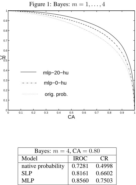
Results obtained for various length predictions of up to four words using the Bayes models are summarized in figure (1)and in table 1 below, and are encouraging. At a fixed CA of0.80we obtain CR increases from0.6604for the native probability to0.7211for the SLP and0.7728 for the MLP. The over-all gain is also evident from the the relative improvements in IROC obtained by the SLP and MLP models over the native probability, that are re-spectively17.06% and33.31%. These results are quite significant.

Note that the improvements obtained in the fixed-length 4-word-prediction tasks with the Bayes model (fig-ure (2) and table 2) model are even larger: the relative improvements on IROC are32.36%and50.07%for the SLP and the MLP, respectively.

However, the results obtained in the Maxent models are much less positive: the SLP CR actually drops, while the MLP CR only increases slightly to a4.80%relative

2

Training and testing of the neural nets was done us-ing the open-source Torch toolkit ((Collobert et al., 2002), http://www.torch.ch/), which provides efficient C++ implemen-tations of many ML algorithms.

Figure 1: Bayes:m= 1, . . . ,4

0 0.1 0.2 0.3 0.4 0.5 0.6 0.7 0.8 0.9 1

0 0.1 0.2 0.3 0.4 0.5 0.6 0.7 0.8 0.9 1

CA CR

mlp−20−hu

mlp−0−hu

orig. prob.

Bayes:m= 4, CA= 0.80

Model IROC CR

native probability 0.7281 0.4998

SLP 0.8161 0.6602

MLP 0.8560 0.7503

Table 2: Comparison of discrimination capacity between the Bayes prediction model probability and the CE of the corresponding SLP and MLP on fixed-length predictions of four words

Figure 2: Bayes:m= 4

0 0.1 0.2 0.3 0.4 0.5 0.6 0.7 0.8 0.9 1

0 0.1 0.2 0.3 0.4 0.5 0.6 0.7 0.8 0.9 1

CA CR

mlp−20−hu

mlp−0−hu

Maxent1:m= 1, . . . ,4, CA= 0.80

Model IROC CR

native probability 0.8581 0.7467

SLP 0.8401 0.7142

MLP 0.8636 0.7561

Table 3: Comparison of discrimination capacity between the Maxent1 prediction model probability and the CE of the corresponding SLP and MLP on predictions of up to four words

Maxent2:m= 1, . . . ,4, CA= 0.80

Model IROC CR

native probability 0.8595 0.7479

SLP 0.8352 0.6973

MLP 0.8638 0.7599

Table 4: Comparison of discrimination capacity between the Maxent2 prediction model probability and the CE of the corresponding SLP and MLP on predictions of up to four words

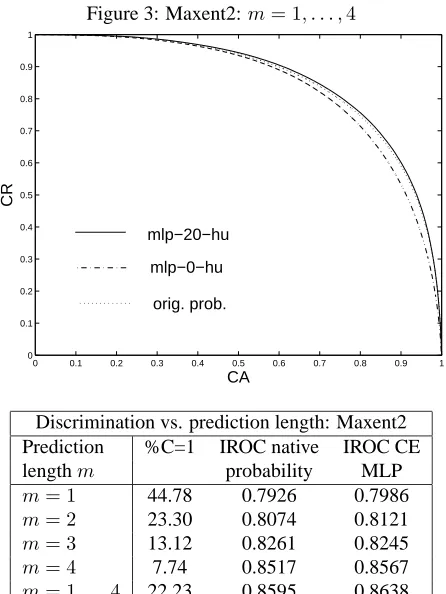
improvement in the CR rate for the Maxent1 model ( ta-ble 3) and only3.9%for the Maxent2 model ( table 4). The results obtained with the two Maxent models are very similar. We therefore only draw the ROC curve for the Maxent2 model (figure (3).

It is interesting to note that the native model predic-tion accuracy didn’t affect the discriminapredic-tion capacity of the corresponding probability of correctness of the CE models. This result is illustrated in table below, where %C = 1 is the percentage of correct predictions. Even though the Bayes’ model accuracy and IROC is signifi-cantly lower then the Maxent model’s, the CE IROC val-ues are almost identical.

6.2 Relevance of Confidence Features

We investigated the relevance of different confidence fea-tures by using the IROC values of single-feature models for the 1–4 word prediction task, with both Maxent1 and Bayes base models.

The group of features that performs best over both models are the model- and search-dependent features de-scribed above, followed by the features that capture the intrinsic difficulty of the source sentence and the target-prefix. Least valuable are the remaining features that capture translation difficulty. The single most significant feature is native probability, followed by the probability ratio of the best hypothesis, and the prediction length. Somewhat unsurprisingly, the weaker Bayes models are much more sensitive to longer translations than the Max-ent models.

Figure 3: Maxent2:m= 1, . . . ,4

0 0.1 0.2 0.3 0.4 0.5 0.6 0.7 0.8 0.9 1

0 0.1 0.2 0.3 0.4 0.5 0.6 0.7 0.8 0.9 1

CA

CR

mlp−20−hu

mlp−0−hu

orig. prob.

Discrimination vs. prediction length: Maxent2 Prediction %C=1 IROC native IROC CE

lengthm probability MLP

m= 1 44.78 0.7926 0.7986

m= 2 23.30 0.8074 0.8121

m= 3 13.12 0.8261 0.8245

m= 4 7.74 0.8517 0.8567

m= 1, ...,4 22.23 0.8595 0.8638

Table 5: Impact of prediction length on discrimination capacity and accuracy for the Maxent2 prediction model

6.3 Dealing with predictions of various lengths

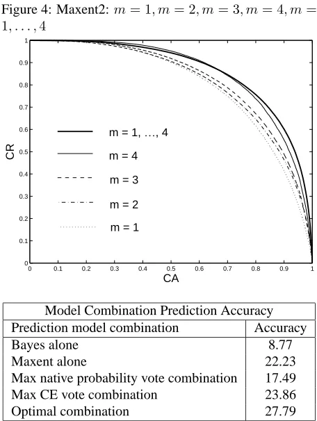
We compared different approaches for dealing with vari-ous length predictions: we trained four separate MLPs for fixed length predictions of one through four words; and a single MLP over predictions of varying lengths. Results are given in table 5 and figure (4)

7

Model Combination

In this section we describe how various model combi-nations schemes affect prediction accuracy. We use the Bayes and the Maxent2 prediction models: we try to ex-ploit the fact that these two models, being fundamentally different, tend to be complementary in some of their re-sponses. The CE models we use are the corresponding MLPs, as they clearly outperform the SLPs. The results presented in table 6 are reported on the variable-length prediction task for up to four words.

The combination schemes are the following: we run the two prediction models in parallel and choose one of the proposed prediction hypotheses according to the fol-lowing voting criteria:

Figure 4: Maxent2:m= 1, m= 2, m= 3, m= 4, m= 1, . . . ,4

0 0.1 0.2 0.3 0.4 0.5 0.6 0.7 0.8 0.9 1

0 0.1 0.2 0.3 0.4 0.5 0.6 0.7 0.8 0.9 1

CA

CR

m = 1 m = 2 m = 3 m = 4 m = 1, …, 4

Model Combination Prediction Accuracy

Prediction model combination Accuracy

Bayes alone 8.77

Maxent alone 22.23

Max native probability vote combination 17.49

Max CE vote combination 23.86

Optimal combination 27.79

Table 6: Prediction accuracy of the Bayes and Maxent2 model compared with combined model accuracy

• Maximum native probability vote: choose the pre-diction with the highest native probability.

As a baseline comparison, we use the accuracy of the individual native prediction models. Then we compute the maximum gain we can expect with an optimal model combination strategy, obtained by running an ”oracle” that always picks the right answer.

The results are very positive: the maximum CE voting scheme obtains a29.31%of the maximum possible ac-curacy gain over the better of the two indiviual models (Maxent2). Moreover, if we choose the maximum native probability vote, the overall accuracy actually drops sig-nificantly. These results are a strong motivation for our post-prediction confidence estimation approach: by train-ing an additional CE layer ustrain-ing the same confidence fea-tures and training data for different underlying prediction models we obtain more uniform estimates of the proba-bility of correctness.

8

User-Model Evaluations

As described in section 2, we evaluated the prediction system as a whole by simulating the actions of a trans-lator on a given source text and measuring the gain

model base mults SLP MLP best

Bayes 3.2 6.5 6.4 6.4 11.8

ME1 16.6 16.5 18.1 18.3 23.5

ME2 17.4 17.4 19.0 19.3 24.3

Table 7: Percentage of typing time saved for various CE configurations.

with a user model. In order to abstract away from ap-proximations made in deriving character-based proba-bilitiesp(k|x,h,s)used in the benefit calculation from word-based probabilities, we employed a specialized user model. In contrast to the realistic model described in (Foster et al., 2002b), this assumes that users accept pre-dictions only at the beginnings of words, and only when they are correct in their entirety. To reduce variation fur-ther, it also assumes that the user always accepts a correct prediction as soon as it is suggested. Thus the model’s estimates of benefit to the user may be slightly over-optimistic: the limited opportunities for accepting and editing must be balanced against the user’s inhumanly perfect decision-making. However, its main purpose is not realism but simply to allow for a fair comparison be-tween the base and the CE models.

Simulations with all three translation models were per-formed using a 500-sentence test text. At each prediction point, the benefits associated with best predictions of 1–4 words in length were compared to decide which (if any) to propose. The results, in terms of percentages of typing time saved, are shown in table 8: base corresponds to the base model; mults to length-specific probability multipli-ers tuned to optimize benefit on a held-out corpus; SLP and MLP to CE estimates; and best to using an oracle to pick the length that maximizes benefit.

Although the CE layer provides no gain over the much simpler probability-multiplier approach for the Bayes model, the gain for both maxent models is substantial, around 10% in relative terms and 25% of the theoretical maximum gain (over the base model) with the MLP and slightly lower with the SLP.

9

Conclusion

The results obtained in this paper can be summarized in the following set of questions and answers:

un-derlying SMT application using confidence estima-tion? In simulated results, we found a significant gain (10% relative) in benefit to a translator due to the use of a CE layer in two of three translation mod-els tested.

• Can prediction accuracy of the application be im-proved using prediction model combinations? A maximum CE voting scheme yields a 29.31% curacy improvement of the maximum possible ac-curacy gain. A similar voting scheme using native probabilies significantly decreases the accuracy of the model combination.

• How does the prediction accuracy of the native mod-els influence the CE accuracy? Prediction accuracy didn’t prove to be a significant factor in determining the discrimination capacity of the confidence esti-mate.

• How does CE accuracy change with various ML ap-proches? A multi-layer perceptron (MLP) with 20 hidden units significantly outperformed one with 0 hidden units (equivalent to a maxent model for this application).

• Confidence feature selection: which confidence fea-tures are more useful and how does their discrimi-nation capacity vary with different contexts and dif-ferent native SMT models? Confidence features based on the original model and the n-best predic-tion turned out to be the most relevant group of fea-tured, folowed by features that capture the intrinsic difficulty of the source text and finally translation-difficulty-specific features. We also observed inter-esting variations in relevance as the original models changed.

Future work will include the search for more relevant confidence features, such as features based on consenus over word-lattices ((Mangu et al., 2000)), past perfor-mance, the use of more appropriate correct/false tagging methods and experiments with different machine learning techniques. Finally, we would like to investigate whether confidence estimation can be used to improve the model prediction accuray, either by using re-scoring techniques or using the confidence estimates during search (decod-ing).

References

Christopher M. Bishop. 1995. Neural Networks for Pat-tern Recognition. Oxford.

Peter F. Brown, Stephen A. Della Pietra, Vincent Della J. Pietra, and Robert L. Mercer. 1993. The mathematics

of Machine Translation: Parameter estimation. Com-putational Linguistics, 19(2):263–312, June.

R. Collobert, S. Bengio, and J. Mari´ethoz. 2002. Torch: a modular machine learning software library. Techni-cal Report IDIAP-RR 02-46, IDIAP.

George Foster, Philippe Langlais, and Guy Lapalme. 2002a. Text prediction with fuzzy alignments. In Stephen D. Richardson, editor, Proceedings of the 5th Conference of the Association for Machine Transla-tion in the Americas, Tiburon, California, October. Springer-Verlag.

George Foster, Philippe Langlais, and Guy Lapalme. 2002b. User-friendly text prediction for translators. In Proceedings of the 2002 Conference on Empirical Methods in Natural Language Processing (EMNLP), Philadelphia, PA.

George Foster. 2000. Incorporating position infor-mation into a Maximum Entropy / Minimum Di-vergence translation model. In Proceedings of the 4th Computational Natural Language Learning Work-shop (CoNLL), Lisbon, Portugal, September. ACL SigNLL.

Didier Guillevic, Simona Gandrabur, and Yves Nor-mandin. 2002. Robust semantic confidence scoring. In Proceedings of the 7th International Conference on Spoken Language Processing (ICSLP) 2002, Denver, Colorado, September.

L. Mangu, E. Brill, and A. Stolcke. 2000. Finding con-sensus in speech recognition: word error minimization and other applications of confusion networks. Com-puter Speech and Language, 14(4):373–400.

R. Manmatha and H. Sever. 2002. A formal approach to score normalization for meta-search. In M. Mar-cus, editor, Proceedings of HLT 2002, Second Inter-national Conference on Human Language Technology Research, pages 98–103, San Francisco. Morgan Kauf-mann.

P. Moreno, B. Logan, and B. Raj. 2001. A boosting approach for confidence scoring. In Eurospeech.

A. Sanchis, A. Juan, and E. Vidal. 2003. A simple hy-brid aligner for generating lexical correspondences in parallel texts. In ICASSP 2003, pages 29–35.

A. Stolcke, Y. Koenig, and M. Weintraub. 1997. Explicit word error minimization in n-best list rescoring. In Proc. 5th Eur. Conf. Speech Communication and Tech-nology, volume 1, pages 163–166.