Abstract—Evolutionary algorithms can efficiently solve multi-objective optimization problems (MOPs) by obtaining diverse and near-optimal solution sets. However, the performance of multi-objective evolutionary algorithms (MOEAs) is often limited by the suitability of their corresponding parameter settings with respect to different optimization problems. The tuning of the parameters is a crucial task which concerns resolving the conflicting goals of convergence and diversity. Moreover, parameter tuning is a time-consuming trial-and-error optimization process which restricts the applicability of MOEAs to provide real-time decision support. To address this issue, we propose a self-adaptive mechanism (SAM) to exploit and optimize the balance between exploration and exploitation during the evolutionary search. This “explore first and exploit later” approach is addressed through the automated and dynamic adjustment of the distribution index of the simulated binary crossover (SBX) operator. Our experimental results suggest that SAM can produce satisfactory results for different problem sets without having to predefine/pre-optimize the MOEA’s parameters. SAM can effectively alleviate the tedious process of parameter tuning thus making on-line decision support using MOEA more feasible.
Index Terms— Self-adaptive, parameter tuning, simulated binary crossover, evolutionary algorithm.
I. INTRODUCTION
Evolutionary algorithms can efficiently solve multi-objective optimization problems (MOPs) by obtaining diverse and near-optimal solution sets. Multiple evolutionary techniques have been proposed for MOPs. Among them, Non-dominated Sorting Genetic Algorithms II (NSGA-II) [1] and Strength Pareto Evolutionary Algorithm II (SPEAII) [2] are commonly regarded as the state-of-the-art multi-objective evolutionary algorithms (MOEAs).
In MOEAs, crossover and mutation operators are typically utilized to produce offspring solutions from selected parent individuals. Both operators involve parameters which dictate: 1. The frequency (crossover and mutation rate) of the
evolutionary operations.
2. The spread (crossover and mutation distribution index) of offspring solutions.
Both the frequency and spread properties govern the conflicting convergence and diversity dynamics of the
Self-Adaptive Mechanism for Multi-objective
Evolutionary Algorithms
Fanchao Zeng, Malcolm Yoke Hean Low, James Decraene, Suiping Zhou, Wentong Cai
Manuscript received 30 December 2009. This work was supported by Defence Science and Technology Agency (DSTA), Singapore.
Zeng Fanchao, Malcolm Yoke Hean Low, James Decraene, Suiping Zhou, and Wentong Cai are with the Parallel and Distributed Computing Centre, School of Computer Engineering, Nanyang Technological University, Nanyang Avenue, Singapore 639798 (phone: 65-65132178; e-mail: {fczeng, yhlow, jdecraene}@ntu.edu.sg).
evolutionary process. Consequently, the performance of MOEAs depends on the suitability of the above parameters setting with respect to specific optimization problems. The tuning of these parameters is thus a critical time-consuming optimization process. As a result, this limits the applicability of MOEAs to provide online decision support for real life problems.
To address this issue, we propose a novel self-adaptive mechanism (SAM) which aims at improving the MOEA’s performance (when applied to different optimization problems) through automatically adjusting/balancing the exploration and exploitation of candidate solutions during the evolutionary search. SAM can dynamically adjust the distribution index of SBX operator in NSGA-II. Identifying a suitable distribution index (ŋc) enables NSGA-II to optimize
the balance between exploration and exploitation during the different stages of the evolutionary search.
The essential idea of SAM is that if the diversity running performance is poor, strong evolutionary operation should be applied to break the clusters of candidate solutions and vice versa. Also, the crowding distance is an estimate of the surrounding density of a given solution point and it could be regarded as a criterion to determine the value of this solution. Hence, if the crowding distance is relatively high, soft evolutionary operation is required to preserve the solution points.
The remainder of the paper is structured as follows: A description of related work is first presented. This is followed with an introduction to the SBX operator and diversity running performance metric. Then, a detailed description of the self-adaptive mechanism is provided. A series of experiments involving multi-objective optimization problems are conducted and discussed. Our conclusion and future work are then finally outlined.
II. RELATED WORK
Past studies [3, 4] have proven the efficiency of the “explore first and exploit later” concept which relies on the intensive exploration of candidate solutions during the early stage and local fine-tuning during the later/final stage of the search.
[3] defined a deterministic-scheduled decreasing mutation rate and also implemented an adaptive variation operator that facilitated the exchange of search information in MOPs [6]. These self-adaptation approaches demonstrated significant improvements over static counterparts; note that these methods focused on the effects of changing the crossover/mutation rates (i.e., frequency) instead of the distribution index parameter (i.e., spread). Here we propose a complementary investigation examining the effects of the spread property.
To our knowledge, the only significant reported study addressing spread was carried out by Deb et al. [7], in which a self-adaptive SBX (SA-SBX) was introduced to dynamically adjust (at each generation) the distribution index of SBX in NSGA-II. SA-SBX was found to produce better results on both single and multiple objective optimization problems compared to the SBX with fixed value of the distribution index. Nevertheless, a drawback of SA-SBX is that it requires another critical user-predefined parameter α. According to the experiments reported in [7], SA-SBX would outperform the traditional non self-adaptive counterpart only when α is manually “well tuned”.
Although the Deb et al.’s approach demonstrated better performances, their method introduced an additional difficulty in the already complex parameter tuning process. Consequently such approaches do not resolve the robustness and applicability issues of MOEAs for real-time applications. In contrast with Deb et al.’s approach, we propose a self-adaptive method which does not introduce another critical parameter to be predefined by the user. This self-adaptive mechanism is presented in the next section.
III. SELF-ADAPTIVE MECHANISM
The working principles of SBX are described to emphasize the importance of distribution index ŋc in generating the
offspring solutions. Then, the implementation details of the diversity running performance metric are presented and the concept of crowding distance is introduced. Finally, we present the self-adaptive mechanism (SAM) which can dynamically adjust the distribution index in SBX using the feedback information from both the diversity running performance metric and the crowding distance.
A. Simulated Binary Crossover (SBX)
The SBX crossover operator [8] creates two offspring solutions (represented as real values) from two selected parent solutions. The procedure of deriving offspring solutions xi(1,t+1)and xi(2,t+1)from the parent solutions xi(1,t) and xi(2,t) is as follow.
A random number is generated. Given a pre-specified probability distribution function (Eq. 1), the value of βi (mathematical definition of βi, see Eq. 9) is
determined so that the area under the probability curve from zero to βi is equal to u. The distribution index ŋc is a
non-negative real number. Figure 1 illustrates the probability density function for creating offspring solutions using the SBX operator from two example parents xi (1,t) =3 and xi (2,t) =6
with distribution index of ŋc =2.0 and ŋc =5.0. Larger values
of ŋc are more likely to produce “near parent” solutions
whereas smaller values of ŋc lead to a more diverse search.
After obtaining βi from Eq. 2, the offspring solutions are
[image:2.595.310.525.53.221.2]calculated using Eq. 3 and 4.
Figure 1: The probability density function for creating offspring solutions with the SBX operator (adapted from [7]).
0,1
0.5 ŋ 1 ŋ , if 1;
0.5 ŋ 1 ŋ1 , otherwise. 1
2 ŋ , 0.5; 1
2 1 ŋ
, 0.5.
2
, 0.5 1 , 1 ,
, 0.5 1 , 1 , 4
3
B. Diversity Running Performance Metric
A modified diversity running performance metric is implemented to dynamically assess the diversity performance of the generated solution sets. This diversity running performance metric is based on the running performance metrics proposed by Deb et al. [9]. Two principal modifications are introduced:
1. The number of grids (approximating the diversity of the population, see Fig. 2) is derived by dividing the population size by the number of objectives (instead of requiring the user to manually define it).
2. Deb et al.’s approach is limited by the requirement of a priori knowledge of the target solutions distribution. Using this information, the number of grids can be determined/fitted. Nevertheless in real time/life optimization problems, this information is usually unavailable. Here the running metric does not refer to any pre-specified target set of solution points. Instead the running metric is employed to converge towards an ideal target set of solutions where each grid would possess a representative solution point.
Step 1: Calculate diversity array.
The number of integer variables in the diversity array is equal to the number of grids in the hyperplane. Each variable in the diversity array corresponds to one particular grid i. The value
h(i) of the ith elements is derived using Eq. 5.
1, ;
0, . 5
Step 2: Assign a value, m() to each grid i depending on its neighboring grids’ h() values in the diversity array. The value of the ith grid is calculated as shown in Table 1.
Table 1: Mapping table to assign a value to m(). (adapted from [9])
h(i-1) h(i) h(i+1) m( h(i-1), h(i), h(i+1) )
0 0 0 0.00
0 0 1 0.50
1 0 0 0.50
0 1 1 0.67
1 1 0 0.67
0 1 0 0.75
1 0 1 0.75
1 1 1 1.00
For example let us consider the grid patterns p1=|0|1|0| (i.e.,
[image:3.595.60.278.248.343.2]h(i-1)=0, h(i)=1 and h(i+1)=0 and p2=|1|0|1|. According to
Table 1, we obtain m(p1) = m(p2) = 0.75 which represent a
good periodic spread pattern. Whereas if we consider
p3=|1|1|0|, we obtain m(p3)= 0.67 meaning that the p3 covers a
smaller spread.
Step 3: For each objective, calculate the diversity measure dm by averaging the m() values.
6
1 0.67 0.50 0.50 0.67 1
5
∑ 1 , , 1
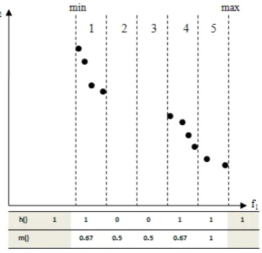
To illustrate the procedure to calculate the diversity measure, an example is presented in Figure 2.
Figure 2: Example of computing the diversity metric.
In this example, a two-objective (f1 and f2) minimization
problem is examined. The solution points are marked as points. The f2 = 0 plane is used as the reference plane and the
range of f1 values are divided into, suppose the population
size is 10, 10/2 = 5 grids. Then, for each grid, the value of h()
is calculated based on whether the grid contains a representative solution point or not. Then, the value of m()
and the diversity measure are calculated based on a sliding window containing three consecutive grids. The h() values of the imaginary boundary grids are always 1 as shown in the shaded grids.
0.668
∑
Step 4: Calculate overall diversity performance metric by averaging the diversity measures of all objective spaces.
7
Figure 3 illustrates the running diversity metric obtained using NSGA-II with population size=100, crossover distribution index ŋc=20.0, mutation distribution index
ŋm=50.0, crossover probability pc=1.0, mutation probability pm=1/30 and 1/10 for the benchmark problems ZDT1 and
ZDT6 respectively, and maximum number of generations
g=500. For ZDT1, after the 100th generation, the diversity
metric oscillates around a value of 0.85. In ZDT6 case, this diversity metric reaches steady state after 160 generations. Similar observations have been reported in Laumanns et al.
[10]. In our implementation, this diversity running performance metric is used to return feedback about the search space. Once the diversity metric stabilizes (i.e., when the exploration phase terminates) the exploitation phase may initiate.
0.5 0.55 0.6 0.65 0.7 0.75 0.8 0.85 0.9 0.95 1
0 50 100 150 200 250 300 350 400 450 500
Div
ersity
Metric
Ev
al
uati
on
ZDT1 ZDT6
[image:3.595.310.543.424.553.2]Number of Generation
Figure 3: Diversity metric dynamics for ZDT1 and ZDT6 using NSGA-II.
C. The Crowding Distance
[image:3.595.79.264.553.731.2]The crowding distance indicator was proposed by Deb et al. [1]. It serves as an estimation of the size of the largest cuboid enclosing the solution point.
[image:3.595.324.541.650.773.2]It could be regarded as a criterion to determine the value of the solution point. In this scheme, “boundary solutions” or highest and lowest objectives are given the maximum value in order to retain them. The crowding distance can be calculated by measuring the distance between the two immediate neighbors of a given point along each of the objective dimensions. Lastly, the “final crowding distance” is computed by adding the crowding distances obtained for each objective. Figure 4 shows a two-objective example illustrating the crowding distance technique. The crowding distance for point i can be computed as follows:
Crowding distance for 8
ŋ
1 1
1
2, 1 1, 1
2,t 1,
D. Self-Adaptive SBX
In most applications of NSGA-II, the crossover rate and mutation distribution index ŋc and ŋm are fixed. Specifically, a
fixed value of ŋc=2.0 is typically chosen for single-objective
optimization problems [11]. Whereas ŋc=20.0 is commonly
used for ZDT benchmark problem sets. Although using a fixed value of ŋc can also lead to the implementation of
self-adaptive techniques, past studies using the SBX operator with fixed distribution index could not solve multi-modal problems such as the Rastrigin’s function [8].
We suggest a self-adaptive mechanism to dynamically update ŋc. Here we assume that for MOPs, the optimal
diversity performance could only be achieved when the solution set is close to the optimal solution set. Hence, if optimal diversity performance is achieved, the distribution index ŋc should be large enough to make the offspring
solutions very similar to their parents. On the other hand, if the diversity performance is poor, strong crossover operation should be applied to break the clusters of solution points. In the beginning stage of the search process, relatively low diversity metric results in strong crossover operation to explore the search space and in the later stage, soft crossover operation is applied to exploit local near-optimal solutions. Thus, this diversity-driven SAM can effectively exploit the concept of “explore first and exploit later”.
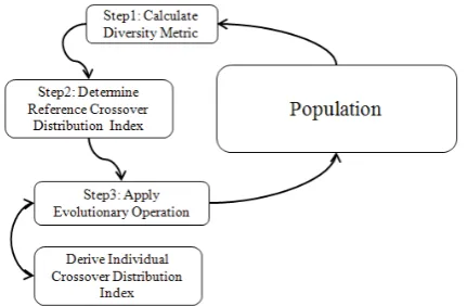
[image:4.595.307.551.299.411.2]Also, a large crowding distance means that the surrounding density of the solution point is low, consequently soft crossover operation should be applied to preserve it. Figure 5 provides an overview of SAM.
Figure 5: Schematic overview of SAM. Firstly, the diversity running performance metric is calculated. Then, a reference distribution index is derived based on the diversity performance of the solution set. Lastly, according to the crowding distances of the selected parents, individual crossover index is assigned to improve the efficiency and accuracy of the crossover operator.
The above SAM algorithm is now detailed:
Step 1: Calculate the diversity running performance metric (Section III.B).
Step 2: Derive the reference crossover distribution index based on the diversity performance.
The spread of the offspring solution points with respect to the parent points is obtained in Eq. 9. Based on , crossover can be classified into three classes, namely contracting crossover ( ), stationary crossover ( ), and expanding crossover ( ). The expanding crossover can “expand” the parent points to form more diverse the offspring points. Contracting crossover has the opposite effect of contracting the parent points. We define the value range of from 0.9 to 1.1 as the close value range (CVR) where the generated offspring solutions are very similar to parent solutions. This range was determined based on parametric studies (more details in next section).
9
0.9,1.1 equals to
ha
ŋ
Figure 6: Mapping between and u value in SAM.
Here we determine the reference distribution index ŋc such
that the probability of falling into the CVR i. e. ,
the diversity performance metric as illustrated in Figure 6. For example, if the diversity running performance metric is 0.70, then we should make sure that 70% of the time 0.9,1.1 . By mapping the random number u to (using Eq. 2), we ve 0.15,0.85. Then ŋc can be calculated using Eq. 10 and 11:
log 2u
log 1, u 0.5; 10
1 log 2 1 u
log , u 0.5. 11
. .
ŋ 1 10.42 and
ŋ 1 .. respectively.
he distribution indexes ŋ 10.42 and ŋ 11.63 are
reference ver distrib
11.63
T
averaged and we obtain a crosso ution index ŋ = 11.0 to produce offspring solutions.
Randomly initialized population causes poor diversity performance at the beginning and consequently lowers the probability of falling into CVR. In the later stage, the diversity performance stabilizes at a relatively higher value and the exploitation phase starts as the probability of
[image:4.595.68.284.586.727.2]St 3: According to the crowding distances cd of the
or each generated offspring solution, individual crossover
ŋ ŋ
2 ep
selected parents, individual crossover distribution indexes are assigned to improve the efficiency and accuracy of the crossover operator.
F
indexes are computed using the expression below.
12
here cd1 and cd2 are the crowding distances of the two
w
selected parents and is the average crowding distance of the entire population. As devised in the crowding distance scheme, the boundary solutions have maximum values. Consequently these values are not included in the calculation of the average crowding distance. Instead, offspring solutions having boundary solutions as parent points are assigned with the highest distribution index to retain them. Following the previous example, ŋc = 11.0 and the crowding distances of the
two parents of offspring solution c are 0.65 and 0.95 respectively with an average crowding distance of 0.50. Given Eq. 12, we have:ŋ′ 11.0
.
. 17.6.
IV. EXPERIMENTS
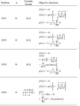
The benc and 6 (Table 2) are
us
athematical definition for the ZDT benchmark problems.
n Variable Objective functions hmark problems ZDT1, 2, 3, 4
ed to evaluate the performance of NSGA-II using SAM. The following parameter setting is used: ŋc = 20.0, ŋm = 50.0, pc = 1.0, pm = 1 / (number of variables). Each set of
[image:5.595.299.552.51.124.2]experiments (where 100,000 fitness evaluations are conducted) is repeated ten times.
Table 2: M
Problem bounds
ZDT1 0 0,1
1 1
2 1 1
3
1 9
1
DT2 0 0,1
1 1
2 1 1
Z 3
1 9
1
ZDT3 30 0,1
1 1
2
1 1
1
sin 10 1
1 9
1
ZDT4 10
1 0,1
5,5 , 2, …
1 1
2 1 1
1 10 1
10 cos 4
ZDT6 10 0,1
1 1
2 1 1
1 9
1
Two benchmark metrics, Inverted Generational Distance (IGD) and SPREAD are employed to measure the performance. IGD uses the true Pareto front1 as a reference
and measure the distance of each of the solution points with respect to the front as (13):
∑
13
0
∑ 1
Where is the Euclidean distance between the solution points and the closet member of the true Pareto front. is the number of solution points in the true Pareto front. When
, it indicates that the obtained solution set is in the true Pareto front. The SPREAD indicates the extent of spread among the obtained solutions and is computed as follows.
14
Where and are the Euclidean distances between the boundary solutions (of the obtained solution set). is the Euclidean distance between consecutive solution points. Tables 3 and 4 summarize the experimental results.
Table 3: Results for the Inverted Generational Distance Metric between SAM NSGA-II and NSGA-II.
Inverted Generational Distance (IGD) Metric NSGA-II with SAM NSGA-II Mean Deviation Standard Mean Deviation Standard
ZDT1 1.74E-04 5.10E-06 1.91E-04 1.08E-05 ZDT2 1.79E-04 5.64E-06 1.88E-04 8.36E-06 ZDT3 2.46E-04 7.74E-06 2.59E-04 1.16E-05 ZDT4 1.67E-04 8.02E-06 1.84E-04 9.86E-06 ZDT6 1.51E-04 1.06E-05 1.59E-04 1.24E-05
Table 4: Results for the Spread Diversity Metric between SAM NSGA-II and NSGA-II.
Spread Diversity Metric
NSGA-II with SAM NSGA-II Mean Deviation Standard Mean Deviation Standard
ZDT1 2.92E-01 3.25E-02 3.83E-01 3.14E-02 ZDT2 3.15E-01 2.01E-02 3.52E-01 7.25E-02 ZDT3 7.31E-01 1.20E-02 7.49E-01 1.49E-02 ZDT4 3.27E-01 2.71E-02 3.96E-01 2.94E-02 ZDT6 4.73E-01 2.98E-02 4.80E-01 4.49E-02
As observed in Tables 3 and 4, SAM achieved lower means for both IGD and Spread diversity metrics in all ZDT problem sets compared to NSGA-II with fixed distribution index. Note that no prior parameter-tuning was conducted for the runs using SAM. As depicted in Figure 6, CVR for is defined from 0.9 to 1.1. Differing CRV definitions may result
1 The true Pareto front used in these experiments was taken from the jMetal
[image:5.595.42.303.445.789.2]CVR 0.6,1.4 . and CVR 0.5,1.5 . The complementary experimental condition, settings, an benchmark are same as in pr
in significantly different reference crossover indexes. To explore the effects upon SAM’s performance, we conduct a parametric study of CRV. Again, we use the ZDT benchmark problem sets to measure the effects of different CVR definition. We evaluate SAM with the following CVR definitions: CVR 0.9,1.1 , CVR 0.8,1.2 , CVR
0.7,1.3 ,
d
the evious experiments.
Table 5: Results for the Inverted Generational Distance Metric with different CVR for SAM NSGA-II and NSGA-II.
Inverted Generational Distance (IGD) Metric S
CV NSGA II
AM SAM SAM SAM SAM
R
.5 CVR 4 CVR0 CVR0 CVR0.9
0.5,1 0.6,1. .7,1.3 .8,1.2 ,1.1
ZDT1 -04 E E E-04 1.
E-0 1. E 1.81 E 1.82 -04 1.80 -04
1.80 74 4
91 -04 ZDT2 E-041.78 E-04 1.79 1.72 E1.7 E1.79 E1.
E-04
6
-04 -04 -04 88
ZDT3 2.36 E2. E2.
E-04 2.44 E-04 2.46 E-04 2.44 E-04 46 -04 59 -04 ZDT4 1.78 1.72 1.73 E1.74 1.67
E-1. E E-04 E-04 E-04 -04 04
84 -04 ZDT6 E-041.76 E-04 1.57 E-04 1.57 1.37 E1. E1.
E-04
51
-04 -04 59
ble 6 lts for the Spread D y Met diffe R SAM NSGA-II and NSGA-II.
ead D y Met
Ta : Resu iversit ric with rent CV for
Spr iversit ric
CVR .5 CVR SAM CVR 0 SAM CVR 0. SAM CVR 0.9, NS SAM 0.5,1 SAM
0.6,1.4 .7,1.3 8,1.2 1.1
G II A
ZDT1 E-01 E-01
E-01 2 E 2. E-01 3. E-2.95 2.96 2.77 .98
-01
92 83 01 ZDT2 E-01 2.96 E-01 2.97 2.80
E-2.87 E-01 3.15 E-01 3.52 E-01 01
ZDT3 7.23 7.28 7.32 7.30 7.31
E-01 E-01 E-01 E-01 E-01 E-01
7.49
ZDT4 E-01
E-01 3.64 3.56
E-01
3.61 E-01
3.40
E-01 3.27
3.96 E-01 ZDT6 E-014.96 E-01 4.89 E-01 4.71 4.57 E4.73 E4.80
E-01 -01 -01
Tables nd 6 compare the erforma e of different CV
niti he b olutio re ma in b e
xcept for ZD D a RE
orm s wer ieved specific CRV settings.
Alt the al a with ect to
different benchmark problem sets, all results using S
f d the e N I w xed bu
x. mo es th form f SA rob
inst rent CVR settin
lso note DT3 the al sett
,1.5 relati wide the r op CVRs
T 1 and e Pa ont DT
on-continuous convex with relatively larger search spa
just the distribution index of th
balance
urther investigations are needed to when applied to real-time problems where the
n SAM will also be
im
ibution and exploration in evolutionary multi-objective optimization. European Journal of Operational Research 171 (2), 463-495.
[4] Janikow, C.Z., Mic rimental comparison of
[5] Abbass, H.A., 2002. T adaptive Pareto differential evolution algorithm. In: Proceed Congress on Evolutionary
5 a p nc R the
defi
observe that e
ons. T est s ns a rked old. W can T1, optimal IG nd SP AD perf
ance e ach with
hough optim CVR v ries resp AM outper
inde
orme bas SGA-I ith fi distri tion ust This de nstrat e per ance o M is
[10
aga A
diffe gs.
, we in Z that optim CVR ing
and
0.5
found
is vely r than othe timal for ZD ,2,4 6. Th reto fr of Z 3 is
ce
Com
n
when compared with other ZDT benchmark problems. Hence, a wider CVR may potentially be more suitable to handle non-continuous large search space. Future work may illuminate this issue.
V. CONCLUSION
Utilizing the feedback from diversity running performance metric and the crowding distance, a self-adaptive mechanism
was suggested to dynamically ad
e SBX operator. SAM is able to exploit and control the between exploration and exploitation during the different evolutionary search stages. We demonstrated that SAM can effectively alleviate the tedious process of parameter tuning which is a time-consuming trial-and-error optimization process. On several benchmark problem sets, SAM was found to outperform NSGA-II with fixed distribution index. F
evaluate SAM
Pareto fro t may be dynamic. Finally,
plemented and evaluated in other MOEAs such as the Bee Colony Optimization and Artificial Immune System techniques.
ACKNOWLEDGMENT
This research is supported under Defence Science and Technology Agency (DSTA) grant POD0814214.
REFERENCES
[1] Deb, K., Agrawal, S., Pratap, A., Meyarivan, T., 2002. A fast and elitist multi-objective genetic algorithm: NSGA-II. IEEE Transactions on Evolutionary Computation 6(2), 182-197.
[2] Zitzler, E., Laumanns, M., Thiele, L., 2001. SPEA2: Improving the strength Pareto evolutionary algorithm. Technical Report 103, Computer Engineering and Networks Laboratory (TIK), Swiss Federal Institute of Technolgy (ETH) Zurich, Switzerland.
[3] Tan, K.C., Goh, C.K., Yang, Y.J., Lee, T.H., 2006. Evolving better population distr
halewicz, Z., 1991. An expe
binary and floating point representations in genetic algorithms. In: Proceedings of the 4th International Conference on Genetic Algorithms,
pp. 151-157.
he self-ings of the 2002 Computation, pp. 831-836.
[6] Tan, K.C., Chiam, S.C., Mamun, A.A., Goh, C.K., 2009. Balancing exploration and exploitation with adaptive variation for evolutionary multi-objective optimization. European Journal of Operational Research, 197(2), pp. 701-713.
[7] Deb, K., Karthink, S., Tatsuya, O., 2007. Self-Adaptive Simulated Binary Crossover for Real-Parameter Optimization. In: Proceedings of
9th annual conference on Genetic and evolutionary computation, 1187 – 1194.
[8] Deb, K., Agrawal, S., 1995. Simulated binary crossover for continuous search space. Complex System, 9(2), 115-148.
[9] Deb, K., Jain, S., 2002. Running Performance Metrics for Evolutionary Multi-Objective Optimization. In: Proceedings of the 4th Asia-Pacific
Conference on Simulated Evolution and Learning (SEAL’02), volume 1, pp. 13-20.
] Laumanns, M., Thiele, L., Deb, K., Zitzler, E., 2001. On the convergence and diversity preservation properties of mulit-objective evolutionary algorithms, Technical Report 108, Computer Engineering Networks Laboratory (TIK), Swiss Federal Institute of Technolgy (ETH) Zurich, Switzerland.
[11] Deb, K., Anand, A. Joshi, D., 2002. A computationally efficient evolutionary algorithm for real-parameter optimization. Evolutionary
![Figure 1: The probability density function for creating offspring solutions with the SBX operator (adapted from [7])](https://thumb-us.123doks.com/thumbv2/123dok_us/1304134.660185/2.595.310.525.53.221/figure-probability-density-function-creating-offspring-solutions-operator.webp)