Gravity Currents in Non-rectangular Cross-section
Channels
Tamar Zemach and Marius Ungarish
Abstract—We consider the propagation of a high-Reynolds-number gravity current at the bottom of a horizontal channel
along the horizontal coordinatex. The bottom and top of the
channel are at z = 0, H, and the cross-section is given by
the general −f1(z) ≤ y ≤ f2(z) for 0 ≤ z ≤ H. We use a
one-layer, Boussinesq, shallow-water (SW) formulation to solve the time-dependent motion produced by release from rest of a fixed volume of fluid from a lock. The dependent variables are the position of the horizontal interface, h(x, t), and the
speed (averaged over the area of the current), u(x, t). For a
given geometry f(z), the only input parameter in the
lock-release problem is the height ratioH/h0of ambient to lock. In
general, the solution is obtained by a finite-difference numerical code. Analytical results are derived for the initial dam-break slumping motion, and for the long-time self-similar phase. The model is illustrated for various cross-section shapes: power-law (f(z) =bzα
, whereb, αare positive constants), trapezoidal and
circle-segment. The theoretical results are in good agreement with previously-published experimental data.
Index Terms—gravity currents, shallow-water.
I. INTRODUCTION
A gravity current appears when fluid of one density spreads into a fluid of another density and the propagation is, mainly, in the horizontal direction. Gravity currents occur at a variety of scales throughout nature. Examples include oceanic fronts, avalanches, seafloor turbidity currents, py-roclastic flows, and lava flows (see for example [1]). Most studies have focused on the flow of currents which propagate on the flat bottom (or top) of a rectangular channel. However, gravity currents generated and spreading in channels with non-rectangular cross-sections are realistic configurations in nature (e.g., valleys and rivers), buildings, irrigation systems, and industrial fluid-transport infrastructures. It is therefore of both practical and academic importance to understand and model the effects of this geometrical property on the flow.
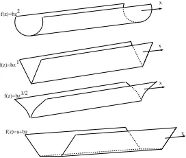
In the present paper we consider gravity currents in channels with various forms of the cross-sections. Typical non-rectangular channels are shown for example in Fig. 1.
Let xbe the horizontal coordinate along the channel,y the
horizontal coordinate orthogonal to x, and z the vertical
coordinate pointing upward. To be specific, the side-walls
are given by y = −f1(z) and y = f2(z), 0 ≤ z ≤ H.
We shall see that the flow depends actually on the width function,f(z) =f1(z)+f2(z), which is assumed continuous
and positive (zero width at0 and/orH are allowed).
Our investigation uses a one-layer shallow-water (SW), Boussinesq model. The formulation is in terms of the height
h of the interface and speed u (averaged over the area of
Manuscript received March 21, 2013
T. Zemach is with the Department of Computer Science, Tel-Hai College, Tel-Hai, Israel, e-mail: [email protected] .
M. Ungarish is with Department of Computer Science, Technion, Haifa 32000, Israel, e-mail:[email protected].
f(z)=bz
f(z)=bz
f(z)=a+bz
2
1/2
f(z)=bz1
x
x
x
[image:1.595.359.495.190.305.2]x
Fig. 1. Schematic description of typical channels with non-rectangular cross-section.
the current) as functions ofxand t (time). This allows the
calculation of the position of the nose,xN(t).
The formulation which we derive is applicable to a quite general cross-section functionf(z)(the main formal require-ment is continuity in [0, H], and the obvious f(z) > 0 in
(0, H)). For definiteness, we shall present results for three
types of channels. (A) f(z) = bzα, where b is a positive
constant and0< α≤2. Experiments for this configuration
were presented by [5], for currents released from a full-depth lock. This geometry is referred to as the power-law cross-section. (B)f(z) =c+bzα, wherec is a positive constant,
and b, α are as above. This geometry is referred to as the
curved-trapezoidal cross-section. (C) A circle-sector channel
of radius R, f(z) = √2zR−z2, 0 ≤z ≤ H <2R. The
three types of cross-section considered here are interesting from the academic point of view, and their relevance to industrial and environmental applications seems feasible. They cover a quite wide domain of shapes and provide a fair understanding of the effects associated with deviations from the classical rectangular geometry.
0000000000000000000000 0000000000000000000000 0000000000000000000000 0000000000000000000000 0000000000000000000000 0000000000000000000000 0000000000000000000000 0000000000000000000000 0000000000000000000000 0000000000000000000000 0000000000000000000000 0000000000000000000000 0000000000000000000000 0000000000000000000000
1111111111111111111111 1111111111111111111111 1111111111111111111111 1111111111111111111111 1111111111111111111111 1111111111111111111111 1111111111111111111111 1111111111111111111111 1111111111111111111111 1111111111111111111111 1111111111111111111111 1111111111111111111111 1111111111111111111111 1111111111111111111111
z
H
ρ
z=h(x,t)
x a
ρc
x
N
g (a)
000000000000000000000000000 000000000000000000000000000 000000000000000000000000000 000000000000000000000000000 000000000000000000000000000 000000000000000000000000000 000000000000000000000000000 000000000000000000000000000 000000000000000000000000000 000000000000000000000000000 000000000000000000000000000 000000000000000000000000000
111111111111111111111111111 111111111111111111111111111 111111111111111111111111111 111111111111111111111111111 111111111111111111111111111 111111111111111111111111111 111111111111111111111111111 111111111111111111111111111 111111111111111111111111111 111111111111111111111111111 111111111111111111111111111 111111111111111111111111111
(b)
y z
a
A
y = f (z) g
h
0 0 y =− f (z)
1 2
H
[image:2.595.64.275.78.172.2]Ac
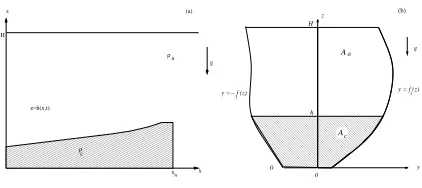
Fig. 2. Schematic description of the gravity current system. (a) Side view. (b) cross-section of channel. Heref(z)is the width of the channel. In the analysisAadenotes the area occupied by the ambient fluid,Ac=F(x, t) is the area occupied by the current, andATis the total area.
II. FORMULATION
The system under consideration is sketched in Fig. 2: a
deep layer of ambient fluid of density ρa and heightH lies
above a horizontal surface at z = 0. Gravity acts in the
−z direction. At time t = 0 a given volume of fluid of
densityρc> ρa(the dark region in the figure), initially at rest
in reservoir of height h0, lengthx0 and same cross-section
as the channel, is instantaneously released into the ambient
fluid. We use a {x, y, z} Cartesian coordinate system with
corresponding {u, v, w} velocity components. We assume
that the fluids are separated by a sharp, non-entraining, interface which is flat (horizontal) in they direction. This is the initial hydrostatic situation in a simple lock. The present model assumes that viscous, turbulent, and entrainment ef-fects are negligible, and hence in the subsequent flow in a straight channel there are no effects that can generate a significant inclination in they direction.
The driving force is the reduced gravity, which is defined by
g′
=ǫg, (1)
wheregis the gravitational acceleration andǫis the reduced
density which is defined by
ǫ=|ρc−ρa|/ρa. (2)
We introduce the Boussinesq assumption ǫ≪1.
We define F = F(h) to be the cross-section area (also
referred to asAc) occupied by the current
F(h) =F(h(x, t)) =
Z h(x,t)
0
f(z)dz=Ac. (3)
Evidently,F′(h) =f(h).
The volume continuity equation of the current can be readily obtained using geometric considerations, see Fig. 2. In the motionless ambient fluid, the pressure does not depend
on x. Therefore, the hydrostatic balances ∂pi/∂z = −ρig,
wherei=aor c, supplemented by the property of pressure
continuity between the ambient and the current on the
interface z = h(x, t), show that the horizontal pressure
gradient in the current is given by
∂pc
∂x =ρcg
′∂h
∂x. (4)
The momentum equation of the model is obtained by
averaging the inviscid x-momentum balance over the area
Ac, and elimination of the pressure term by (4). After some
algebra, and use of (3)-(4) , this equation can be reduced to exactly the same form as in the classical rectangular- cross-section case (see below (6)).
It is convenient to use dimensionless variables. Here we denote the dimensional variables by asterisks, and transform to the dimensionless counterpart (with no special notation) as follows:
{x∗ , z∗
, h∗ , H∗
, t∗ , u∗
, p∗
}=
=
x0x, h0z, h0h, h0H, T t, U u, ρaU2p ,
(5)
where U = (h0g′)1/2 and T = x0/U. The y-direction
lengths are scaled with the width of the interface in the lock, f(h0).
The resulting dimensionless SW system of equations is
ht
ut
+
u F(h) F′
(h)
1 u
hx
ux
=
0 0
. (6)
The system is hyperbolic, with characteristic relationships given by
dh±
s F(h)
F′(h)du= 0 (7)
on
dx
dt =c±=u± s
F(h)
F′(h). (8)
For a lock-release problem, the initial conditions areu= 0
and given position of the interface (in our case, h= 1) in
the reservoir. The boundary conditions are: (1) the obvious
u= 0 at the backwall x= 0; and (2) Froude condition at
the nosex=xN(t):
u(x=xN) =uN =F r·h1N/2, (9)
where F r is the Froude number for the appropriate
non-rectangular cross-section. As shown by [6], for a givenf(z), this reads
F r=F rU(ϕ) =
2(1
−ϕ)2
1 +ϕ (1 +Q)
1/2
, (10)
where
ϕ=F(h)
AT
, and Q=
Rh
0 zf(z)dz
h·[AT−F(h)]
. (11)
HereAT is the total area of the cross-section, and evidently
ϕ <1.
III. FINITE-DIFFERENCE RESULTS
To complete our modelling task, we need an efficient method for obtaining the h(x, t), u(x, t) andxN(t)results
from our formulation. In general, the system of equations (6)-(10), with realistic initial/boundary conditions, cannot be solved analytically. We use a finite-difference two-step Lax-Wendroff method ( [9], [10]), To facilitate the
imple-mentation of the boundary conditions, thex-coordinate was
mapped into the coordinate η = x/xN(t). The SW results
displayed here were obtained with, typically, 200 grid points in the[0, xN]interval, and time step of1·10−3. (Convergence
was tested also on finer grids.)
0 5 10 15 20 0
0.2 0.4 0.6 0.8 1
x
h
0 5 10 15 20
0 0.2 0.4 0.6 0.8 1
x
u
Fig. 3. Profiles ofhanduvs.tfor various values oft.H= 20,f(z) =z
for t= 2(2)20.
A. Power-law cross-section,f(z) =bzα
The dimensional f(z) = bzα reads f(z) = zα in
dimensionless form (the scaling width is bhα
0). This means
that the value ofb does not influence the results.
The typical behaviour of the time-dependent current is
shown in Fig. 3 forH = 20.0 andα= 1.0.
We can distinguish between three main stages of propa-gation, like in the classical rectangular geometry. The initial slumping stage is characterized by the constant value of the
velocity of the nose uN, accompanied by a constant value
of the nose heighthN. The nose heighthN of the slumping
stage increases with α from 0.4 for α = 0.5 to about 0.5
for α = 2. uN also increases with α, but more like h1N/2,
because F r is close to a constant (≈ √2 ) for this value
of H (not shown here). In the currents under consideration
the slumping stage is quite long: until t≈6.4 for α= 0.5,
t≈8 for α= 1.0 andt≈12.0 for α= 2. The distance of
propagation during this stage increases withαand it attains
xs ≈ 6.4 for α = 0.5, xs ≈ 8.5 for α = 1, xs ≈ 11 for
α= 2. We conclude that asαincreases, the current becomes
faster, and the slumping stage becomes longer.
The next stage of propagation is characterized by the decreasing height of the nose and speed. This stage is a transient during which the current approaches a similarity solution. The transition is smooth and it is therefore not possible to give a clear-cut statement when this intermediary phase ends. The long-time profiles display a tendency to self-similar behaviour, which can be identified by a linear
dependency of the velocityuonx, and a “tail down - nose
up” parabolic form of height h. The similarity solution was
reported by [3], [5], and will be discussed in more details in Section V below.
Additional insights were obtained by further comparison
with solutions for non-deep ambient H = 2.0 (not shown
here). Our main conclusion is that the fastest current is
obtained for the largest tested α, and the slumping height
[image:3.595.361.494.78.165.2]hN and distancexs increase withα.
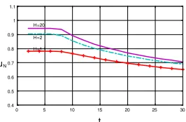
Fig. 4 illustrates the influence of H on the behaviour of
the speeduN as a function of t for the casef(z) =z. The
slumping stage of propagation (with constant uN vs.t) can
be clearly seen on the graph. After the slumping stage, there is a clear-cut tendency of the speed to decrease witht, for all
H. However, the reduction of speed is not sharp:uN decays
by about 20%while tincreases by a factor of more than 3.
In other words, in this case uN decreases less thant−1/5.
uN H=20 H=2 H=1.1
0 5 10 15 20 25 30 0.4
0.5 0.6 0.7 0.8 0.9 1 1.1
[image:3.595.54.285.79.148.2]t
Fig. 4. Numerical results: behaviour of the nose velocity uN vs.tfor
f(z) =zand various values ofH: 1.1, 2.0, and 20.0. Note the constant velocity during the initial (slumping) stage.
0 5 10 15 20
0 0.2 0.4 0.6 0.8 1
x
h
0 5 10 15 20
0 0.2 0.4 0.6 0.8 1
x
u
Fig. 5. Profiles of h and u vs.t for various values of t. H = 20,
f(z) = (1 +z)/2fort= 2(2)20
B. Cross-section withf(z) =c+bzα functions.
The simple (straight planes) trapezoidal case is obtained
forα= 1. For small values ofdwe return to the power-law
case.
The typical behaviour of the solutions is presented in Fig. 5 for H = 20.0 andf(z) = (1 +z)/2 (i.e.,d= 1, α= 1). The current propagation is shown fort= 2,4, ..,20.
We tested and compared results for various parameters for the present configuration. In particular, three values of α were used as before 0.5,1.0,2.0 and two systems: deep
withH = 20, and shallow withH = 2. Ford= 1, the main
conclusions about the tendency of deep (H = 20) currents
to propagate faster than non-deep (H = 2.0) were similar
to these obtained for the d = 0 case and described in the
previous section. The effect ofαon the current is as before:
we see faster propagation for largerα.
C. Circle-sector channel (f(z) =√2Rz−z2 function).
Another interesting and practical configuration is the
circle-sector channel of radiusR.
Here we scale R withh0, and, as an exception, we also
scalef(z)withh0. Therefore,f(z) =
√
2zR−z2, 0≤z≤
H, and obviouslyH <2R. A schematic description of this
configuration is given in Fig. 6.
The typical profiles of the solutions are presented in Fig.
7 for H = 20.0 and R = 10. The current propagation is
shown fort= 2,4, ..,20.
IV. DAM-BREAK AND THE CONSTANT SLUMPINGuN
[image:3.595.310.543.223.292.2]0000000000000000000000000000000 0000000000000000000000000000000 0000000000000000000000000000000 0000000000000000000000000000000 0000000000000000000000000000000 0000000000000000000000000000000 0000000000000000000000000000000 0000000000000000000000000000000 0000000000000000000000000000000 0000000000000000000000000000000 0000000000000000000000000000000 0000000000000000000000000000000 0000000000000000000000000000000 0000000000000000000000000000000 0000000000000000000000000000000 0000000000000000000000000000000 0000000000000000000000000000000 0000000000000000000000000000000 0000000000000000000000000000000 0000000000000000000000000000000 0000000000000000000000000000000 0000000000000000000000000000000 0000000000000000000000000000000 0000000000000000000000000000000 0000000000000000000000000000000 0000000000000000000000000000000 0000000000000000000000000000000 0000000000000000000000000000000 0000000000000000000000000000000 0000000000000000000000000000000 0000000000000000000000000000000 0000000000000000000000000000000 0000000000000000000000000000000 0000000000000000000000000000000 0000000000000000000000000000000 0000000000000000000000000000000 0000000000000000000000000000000 0000000000000000000000000000000 0000000000000000000000000000000 0000000000000000000000000000000 0000000000000000000000000000000 0000000000000000000000000000000 0000000000000000000000000000000 0000000000000000000000000000000 0000000000000000000000000000000 0000000000000000000000000000000 0000000000000000000000000000000 0000000000000000000000000000000 0000000000000000000000000000000 0000000000000000000000000000000 0000000000000000000000000000000 0000000000000000000000000000000 0000000000000000000000000000000 0000000000000000000000000000000 0000000000000000000000000000000 0000000000000000000000000000000 0000000000000000000000000000000 0000000000000000000000000000000 0000000000000000000000000000000 0000000000000000000000000000000 1111111111111111111111111111111 1111111111111111111111111111111 1111111111111111111111111111111 1111111111111111111111111111111 1111111111111111111111111111111 1111111111111111111111111111111 1111111111111111111111111111111 1111111111111111111111111111111 1111111111111111111111111111111 1111111111111111111111111111111 1111111111111111111111111111111 1111111111111111111111111111111 1111111111111111111111111111111 1111111111111111111111111111111 1111111111111111111111111111111 1111111111111111111111111111111 1111111111111111111111111111111 1111111111111111111111111111111 1111111111111111111111111111111 1111111111111111111111111111111 1111111111111111111111111111111 1111111111111111111111111111111 1111111111111111111111111111111 1111111111111111111111111111111 1111111111111111111111111111111 1111111111111111111111111111111 1111111111111111111111111111111 1111111111111111111111111111111 1111111111111111111111111111111 1111111111111111111111111111111 1111111111111111111111111111111 1111111111111111111111111111111 1111111111111111111111111111111 1111111111111111111111111111111 1111111111111111111111111111111 1111111111111111111111111111111 1111111111111111111111111111111 1111111111111111111111111111111 1111111111111111111111111111111 1111111111111111111111111111111 1111111111111111111111111111111 1111111111111111111111111111111 1111111111111111111111111111111 1111111111111111111111111111111 1111111111111111111111111111111 1111111111111111111111111111111 1111111111111111111111111111111 1111111111111111111111111111111 1111111111111111111111111111111 1111111111111111111111111111111 1111111111111111111111111111111 1111111111111111111111111111111 1111111111111111111111111111111 1111111111111111111111111111111 1111111111111111111111111111111 1111111111111111111111111111111 1111111111111111111111111111111 1111111111111111111111111111111 1111111111111111111111111111111 1111111111111111111111111111111 z h H 2R y
Fig. 6. Circle cross-sectionf(z) =√2zR−z2
0 5 10 15 20
0 0.2 0.4 0.6 0.8 1 x h
0 5 10 15 20
0 0.2 0.4 0.6 0.8 1 x u
Fig. 7. Profiles ofhanduvs.tfor various values oft.H= 20,R= 10,
f(z) =√2zR−z2for t= 2(2)20.
We introduce the function
Γ(h) =
Z h
0
s F′(˜h)
F(˜h)d ˜
h. (12)
The integration of the balance equation (7) for u(h) on
a c+ characteristic from the reservoir to the nose and the
intersection of speed dictated by the reservoir, with the nose condition (9) yields:
Γ(1)−Γ(hN) =F r(hN/H)·h1N/2, (13)
where F r is given by (10). The solution of this algebraic
equation provides first hN, and nextuN.
Analytical slumping results for some typical functions f(z)are presented below.
A. f(z) =zα (dimensionless)
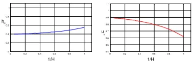
This case allows some analytical progress. A summary of typical analytical results obtained by the abovementioned calculations are presented in Fig. 8. It displays the nose
heighthN and the nose velocityuN as functions of1/Hfor
four values of α: 0,0.5,1.0,2.0. For α≥0,uN increases
with H and the nose height hN decreases with H. It is
interesting to note that all the cases considered here display
the tendency of an increasinguN withH. This is consistent
with the expectations that a deeper current moves faster.
B. f(z) =c+bzα.
The typical solutions are shown in Fig. 9 for the dimen-sionlessf(z) = (d+z)/(d+ 1), whered= 0,1and5. The
effect ofd is interesting: the slumping speed of the current
decreases asdincreases (for any height of the ambient fluid
H). This behavior is, again, in agreement with the numerical
SW solutions obtained above (see for example Fig. 3 and Fig. 5). The interpretation is that, for a givenhN, whendis
hN
0 0.2 0.4 0.6 0.8 1
0 0.2 0.4 0.6 0.8 1 1/H u N
[image:4.595.122.227.79.172.2]0 0.2 0.4 0.6 0.8 1 0.4 0.5 0.6 0.7 0.8 0.9 1 1.1 1/H
Fig. 8. Analytical results for the slumping stage of the current forf(z) =
zα
: Nose height and speed as functions of1/H.α= 2(light blue online) ,α= 1(red online),α= 0.5(green online),α= 0(blue online; this is the classical rectangular case).
u
N
0 0.2 0.4 0.6 0.8 1 0.4 0.5 0.6 0.7 0.8 0.9 1 1.1 1/H
Fig. 9. Analytical slumping speed for trapezoidalf(z) = (d+z)/(d+ 1), whered= 0(upper line, red online),d= 1(blue online),d= 5(black). The lowest line (green online) is for the classical rectangular cross-section.
small, the ratio ofAc to that of the ambient is smaller than
in the rectangular case; therefore the current feels thinner,
and is faster. Thed= 5case is very close to the rectangular
cross-section solution.
C. Circle-sector channel
We focus on the R = 10 case, and let H vary. Fig. 10
displays the nose height hN and the nose velocity uN as
functions of 1/H. Again, the speed uN, increases with H
and the nose heighthN decreases withH. (This means that
F r increases faster than the decrease ofh1N/2.)
We mention here that numerical results of the initial-value
problem were also obtained for deep (H = 20) and shallow
(H = 2) cases with two values of R: 10 and 20. For the
shallow case withH = 2 we obtain that the velocity of the
current decreases for increasing values ofR. ForH = 20, the
numerical results were almost unaffected by these changes of the radiusR. In all cases, the finite-difference results were in excellent agreement with the analytical solution during the slumping stage of propagation.
hN
0 0.2 0.4 0.6 0.8 1 0 0.2 0.4 0.6 0.8 1 1/H u N
0 0.2 0.4 0.6 0.8 1 0.4 0.5 0.6 0.7 0.8 0.9 1 1.1 1/H
Fig. 10. Analytical slumping results for circle segment f(z) = √
2Rz−z2,
[image:4.595.55.286.231.300.2] [image:4.595.385.467.232.291.2] [image:4.595.332.520.680.740.2]V. SIMILARITY SOLUTIONS
Analytical results of self-similar type are also of impor-tance in the study of gravity currents, and it makes sense to ask how this branch of results is affected by the function f(z).
The accepted argument is that, at large times after re-lease, the current is not influenced by the initial conditions. Moreover, in this stage of propagation, the current is already
thin and therefore F r can be considered as constant (=√2
theoretically). In these circumstances, the SW equations are expected to admit a self-similar solution of the form
xN(t) =Ktβ, hN(t, η) = ( ˙xN)2H(η),
uN(t, η) = ˙xNU(η), (14)
where
η= x
xN
; (15)
H(1) = 1/F r2; U(1) = 1. (16)
The upper dot means time derivative, and K and β are
constants.
The formulation above satisfies the nose condition uN =
˙
xN =F r·h1N/2. The remaining details must be obtained from
the other boundary conditions and the equations of motion. The extension to the non-rectangular case is, in general,
problematic. The F r approaches the same constant as in
the classical case. However, the difficulty appears because the area of the current, Ac(h), is in general not a separable
function oftandη. Indeed, [3], [5] have derived, for the SW
equations in power-law cross-sectionsf(z) =zα, similarity
solutions of the form (14). The results, in dimensionless
form, for a current of fixed volume (dimensionless) V =
1/(α+ 1)read
β = 2 + 23 + 2αα , (17)
H(η) = 1
F r2 −
1−η2
4(α+ 1), U(η) =η, (18)
K=
1
β
β 1
R1
0 H
α+1(η)dη
!1/(2α+3)
. (19)
It can be verified by substitution that this solution satisfies the equations (6).
α β K
0 0.667 1.890
0.5 0.750 1.765
1.0 0.800 1.694
2.0 0.857 1.613
TABLE I
SIMILARITY SOLUTION COEFFICIENTS FORf(z) =zα
CROSS-SECTION
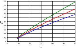
Finally, we verify that the self-similar behavior is indeed attained by the lock-released current. We recall that the finite-difference time-dependent SW solution show the tendency to
approach a “nose up - tail down” parabolic h profile, and
linear with x profile of u, as seen in Fig. 3 More careful
comparisons between the similarity analytical expressions (14) and the finite-difference results are shown in Fig. 11
for f(z) =zα. The values ofK, β used in this comparison
are given in Table 1.
x
N
0 10 20 30 40 50 60
5 10 15 20 25 30 35 40 45 50 55
[image:5.595.361.493.52.136.2]t
Fig. 11. Comparison between analytical similarity solutions (14) (dots) and numerical results of the lock-release current (line) for the cross-sections
f(z) =zα
,α= 0.5,1,2(lower, middle and upper lines; online: blue, red, green).
xN
0 5 10 15 20 25 30 35 40 0
5 10 15 20 25 30
[image:5.595.360.492.226.315.2]t
Fig. 12. Comparison of the experimental results of Monaghan et al. [3] (symbols) and SW prediction (line) forH= 1,f(z) =z.
VI. COMPARISON WITH EXPERIMENTS
It is of course desirable to corroborate the theoretical predictions of the SW model with experimental results. To our best knowledge, the only pertinent available experimental results for non-rectangular cross-sections, of [3], [4], [5], are
for full-depth lock (H= 1) configurations. It is known from
the classical rectangular case that the H = 1 lock-release
produces some special effects which are not captured by the one-layer model (in particular, a backward-moving jump of the interface, and a long slumping interval). This is because the return flow in the ambient plays a significant role. The
experiments of [3] used a tank with V-shaped bottom of5m
length, 0.4m high and 0.28m wide; the slope of inclined
side-walls (f = z) was 25◦
from the horizontal. A gate was located at 0.13m from the rear of the channel. Behind the gate, the container was filled with the aqueous saline solution, while its second part contained fresh water. The
initial height of the both fluids was the same (H = 1). In
the reported experiments the flow was initiated by rapidly lifting the gate.
Fig. 12 presents a comparison between the present SW
results and experimental data reported by [3] for H =
1.0, f(z) =z(experiments 7-10) concerning the position of the nose,xN, as a function oft. The laboratory data is fairly
well predicted by the SW results. During the first stage of
propagation (t .10), the agreement between the one-layer
model and experiments is actually excellent. At later times, the observed propagation lags behind the SW predictions;
however, the discrepancy is only a few percent fort < 27,
when a significant propagation ofxN ≈20 is attained. For
t > 30 the discrepancy becomes more pronounced, and it seems plausible that viscous effects become significant at this stage (consistent with the estimates of [3]).
in spite of the fact that the end of the constant-speed stage
is at t ≈8. This is because in thef(z) = z the decay of
the speed with time is less pronounced than in the classical rectangular case.
The real gravity current is of course more complicated than the SW solution. The observations [3] revealed a parabolic head, and strong billows on the interface. These details are beyond the resolution and the scope of the present model. However, this may indicate that some corrections due to three-dimensional flow components, turbulence, and entrainment are necessary for a more accurate understanding of the real gravity current. Given the paucity of the available experimental data, and the lack of Navier-Stokes simulation, this remains an open question.
VII. CONCLUDING REMARKS
We considered the effect of the shape of the cross-section of the channel on the time-dependent propagation of high-Reynolds-number gravity currents. The cross-section is defined by −f1(z) ≤y ≤f2(z), 0 < z < H; the bottom
z= 0and topz=H walls are straight horizontal planes; the
current propagates over the bottom in direction x. We used
a Boussinesq one-layer shallow-water model, closed by an
analyticalF rconditions at the nose (provided by Ungarish’s
[6] extension of Benjamin’s result). The geometry of the side walls enters the formulation viaf(z) =f1(z) +f2(z). This
model admits quite general forms off(z), and realistic initial and boundary conditions. The governing equations were derived from first principles, without adjustable constants.
We focused attention on currents of fixed volume gen-erated by lock release from rest. For a given cross-section
geometry, the only free input parameter isH, the height ratio
of the ambient to the lock. In general, the time-dependent motion requires numerical solution. We used a simple finite-difference code based on a Lax-Wendroff two-step method. In all the tested cases, the numerical solution of the SW model was obtained within insignificant computational effort on a simple laptop computer.
We also considered analytical solutions of the SW model. We analyzed the dam-break problem, showed that an initial slumping stage with constant speed of propagation appears for any cross-section geometry, and derived a simple formula for this speed. We also revisited the analytical self-similar so-lution presented in previous studies ([3], [5]). We conjectured that such solutions for non-rectangular cross-sections exist
only for the power-law shape f(z) = bzα. We compared
the analytical and numerical SW results, and found good agreement.
We illustrated the application of the SW model for various cross-section forms:f(z) =bzα,f(z) =b(d+zα) and circle
segment.
REFERENCES
[1] J. E. Simpson. Gravity Currents in the Environment and the Labora-tory. Cambridge University Press, Cambridge UK, 1997.
[2] M. Ungarish. An Introduction to Gravity Currents and Intrusions. Chapman & Hall/CRC press, Boca Raton London New York, 2009. [3] J.J. Monaghan, C.A. M´eriaux, H.E. Huppert, and J.M. Monaghan.
High Reynolds number gravity currents along V-shaped valleys. Eu-ropean Journal of Mechanics - B/Fluids, 28(5):651 – 659, 2009. [4] B. M. Marino and L. P. Thomas. Front condition for gravity currents
in channels of nonrectangular symmetric cross-section shapes. Journal of Fluids Engineering, 131(5):051201, 2009.
[5] B. M. Marino and L. P. Thomas. Dam-break release of a gravity current in a power-law channel section. Journal of Physics: Conference Series 296 (2011) 012008, doi: 10.1088/1742-6596/296/1/012008, 2011.
[6] M. Ungarish. A general solution of Benjamin-type gravity current in a channel of non-rectangular cross-section. Environ Fluid Mech., 12(3):251–263, 2011.
[7] T. B. Benjamin. Gravity currents and related phenomena. J. Fluid Mech., 31:209–248, 1968.
[8] T. Bonometti, M. Ungarish, and S. Balachandar. A numerical inves-tigation of constant-volume non-Boussinesq gravity currents in deep ambient. J. Fluid Mech., 673:574–602, 2011.
[9] M. Ungarish and T. Zemach. On the slumping of high Reynolds number gravity currents in two-dimensional and axisymmetric config-urations. European J. Mech. B/Fluids, 24:71–90, 2005.
[10] R. T. Bonnecaze, H. E. Huppert, and J. R. Lister. Particle-driven gravity currents. J. Fluid Mech., 250:339–369, 1993.
[11] D. Takagi and H. E. Huppert. The effect of confining boundaries on viscous gravity currents. J. Fluid Mech., 577:495–505, 2007. [12] T. Zemach and M.Ungarish. Gravity currents in non-rectangular