A Hedgehop over a Max Margin Framework Using Hedge Cues

A Hedgehop over a Max-Margin Framework Using Hedge Cues

Maria Georgescul

ISSCO, ETI, University of Geneva 40 bd. du Pont-d'Arve

CH-1211 Geneva 4

maria.georgescul@unige.ch

Abstract

In this paper, we describe the experimental settings we adopted in the context of the 2010 CoNLL shared task for detecting sentences containing uncertainty. The classification results reported on are obtained using discriminative learning with features essentially incorporating lexical information. Hyper-parameters are tuned for each domain: using BioScope training data for the biomedical domain and Wikipedia training data for the Wikipedia test set. By allowing an efficient handling of combinations of large-scale input features, the discriminative approach we adopted showed highly competitive empirical results for hedge detection on the Wikipedia dataset: our system is ranked as the first with an F-score of 60.17%.

1 Introduction and related work

One of the first attempts in exploiting a Support Vector Machine (SVM) classifier to select speculative sentences is described in Light et al. (2004). They adopted a bag-of-words representation of text sentences occurring in MEDLINE abstracts and reported on preliminary results obtained. As a baseline they used an algorithm based on finding speculative sentences by simply checking whether any cue (from a given list of 14 cues) occurs in the sentence to be classified.

Medlock and Briscoe (2007) also used single words as input features in order to classify sentences from scientific articles in biomedical domain as speculative or non-speculative. In a first step they employed a weakly supervised Bayesian learning model in order to derive the probability of each word to represent a hedge cue. In the next step, they perform feature selection based on these probabilities. In the last step a classifier trained on a given number of

selected features was applied. Medlock and Briscoe (2007) use a similar baseline as the one adopted by Light et al. (2004), i.e. a naïve algorithm based on substring matching, but with a different list of terms to match against. Their baseline has a recall/precision break-even point of 0.60, while their system improves the accuracy to a recall/precision break-even point of 0.76. However Medlock and Briscoe (2007) note that their model is unsuccessful in identifying assertive statements of knowledge paucity which are generally marked rather syntactically than lexically.

Kilicoglu and Bergler (2008) proposed a semi-automatic approach incorporating syntactic and some semantic information in order to enrich or refine a list of lexical hedging cues that are used as input features for automatic detection of uncertain sentences in the biomedical domain. They also used lexical cues and syntactic patterns that strongly suggest non-speculative contexts (“unhedges”). Then they manually expanded and refined the set of lexical hedging and “unhedging” cues using conceptual semantic and lexical relations extracted from WordNet (Fellbaum, 1998) and the UMLS SPECIALIST Lexicon (McCray et al. 1994). Kilicoglu and Bergler (2008) did experiments on the same dataset as Medlock and Briscoe (2007) and their experimental results proved that the classification accuracy can be improved by approximately 9% (from an F-score of 76% to an F-score of 85%) if syntactic and semantic information are incorporated.

The experiments run by Medlock (2008) on the same dataset as Medlock and Briscoe (2007) show that adding features based on part-of-speech tags to a bag-of-words input representation can slightly improve the accuracy, but the “improvements are marginal and not statistically significant”. Their experimental results also show that stemming can slightly

Dataset

#sente nces

%uncertain sentences

#distinct cues

#ambiguous

cues P R F

Wikipedia training 11111 22% 1912 0.32 0.96 0.48

Wikipedia test 9634 23% - 188 0.45 0.86 0.59

BioScope training 14541 18% 168 0.46 0.99 0.63

BioScope test 5003 16% - 96 0.42 0.98 0.59

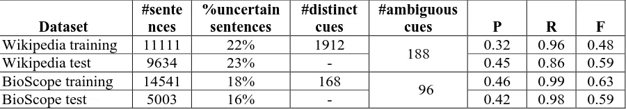
Table 1: The percentage of “uncertain” sentences (% uncertain sentences) given the total number of available sentences (#sentences) together with the number of distinct cues in the training corpus and the performance of the baseline algorithm based on the list of cues extracted from the training corpus.

improve the classification accuracy, while using bigrams brings a statistically significant improvement over a simple bag-of-words representation. However, Medlock (2008) illustrates that “whether a particular term acts as a hedge cue is quite often a rather subtle function of its sense usage, in which case the distinctions may well not be captured by part-of-speech tagging”.

Móra et al. (2009) also used a machine learning framework based on lexical input features and part-of-speech tags. Other recent work on hedge detection (Ganter and Strube, 2009; Marco and Mercer, 2004; Mercer et al., 2004; Morante and Daelemans, 2009a; Szarvas, 2008) relied primarily on word frequencies as primary features including various shallow syntactic or semantic information.

The corpora made available in the CoNLL shared task (Farkas et al., 2010; Vincze et al., 2008) contains multi-word expressions that have been annotated by linguists as cue words tending to express hedging. In this paper, we test whether it might suffice to rely on this list of cues alone for automatic hedge detection. The classification results reported on are obtained using support vector machines trained with features essentially incorporating lexical information, i.e. features extracted from the list of hedge cues provided with the training corpus.

In the following, we will first describe some preliminary considerations regarding the results that can be achieved using a naïve baseline algorithm (Section 2). Section 3 summarizes the experimental settings and the input features adopted, as well as the experimental results we obtained on the CoNLL test data. We also report on the intermediate results we obtained when only the CoNLL training dataset was available. In Section 4, we conclude with a brief description of the theoretical and practical advantages of our system. Future research directions are mentioned in Section 5.

2 Preliminary Considerations

2.1 Benchmarking

As a baseline for our experiments, we consider a naive algorithm that classifies as “uncertain” any sentence that contains a hedge cue, i.e. any of the multi-word expressions labeled as hedge cues in the training corpus.

Table 1 shows the results obtained when using the baseline naïve algorithm on the CoNLL datasets provided for training and test purposes1. The performance of the baseline algorithm is denoted by Precision (P), Recall (R) and F-score (F) measures. The first three columns of the table show the total number of available sentences together with the percentage of “uncertain” sentences occurring in the dataset. The fourth column of the table shows the total number of distinct hedge cues extracted from the training corpus. Those hedge cues occurring in “certain” sentences are denoted as “ambiguous cues”. The fifth column of the table shows the number of distinct ambiguous cues.

As we observe from Table 1, the baseline algorithm has very high values for the recall score on the BioScope corpus (both training and test data). The small percentage of false negatives on the BioScope test data reflects the fact that only a small percentage of “uncertain” sentences in the reference test dataset do not contain a hedge cue that occurs in the training dataset.

The precision of the baseline algorithm has values under 0.5 on all four datasets (i.e. on both BioScope and Wikipedia data). This illustrates that ambiguous hedge cues are frequently used in “certain” sentences. That is, the baseline algorithm has less true positives than false

1

positives, i.e. more than 50% of the sentences containing a hedge cue are labeled as “certain” in the reference datasets.

2.2 Beyond bag-of-words

In order to verify whether simply the frequencies of all words (except stop-words) occurring in a sentence might suffice to discriminate between “certain” and “uncertain” sentences, we performed preliminary experiments with a SVM bag-of-words model. The accuracy of this system is lower than the baseline accuracy on both datasets (BioScope and Wikipedia). For instance, the classifier based on a bag-of-words representation obtains an F-score of approximately 42% on Wikipedia data, while the baseline has an F-score of 49% on the same dataset. Another disadvantage of using a bag-of-words input representation is obviously the large dimension of the system’s input matrix. For instance, the input matrix representation of the Wikipedia training dataset would have approximately 11111 rows and over 150000 columns which would require over 6GB of RAM for a non-sparse matrix representation.

3 System Description

3.1 Experimental Settings

In our work for the CoNLL shared task, we used Support Vector Machine classification (Fan et al., 2005; Vapnik, 1998) based on the Gaussian Radial Basis kernel function (RBF). We tuned the width of the RBF kernel (denoted by gamma) and the regularization parameter (denoted by C) via grid search over the following range of values: {2-8, 2-7, 2-6, …24} for gamma and {1, 10..200 step 10, 200..500 step 100} for C. During parameter tuning, we performed 10-fold cross validation for each possible value of these parameters. Since the training data are unbalanced (e.g. 18% of the total number of sentences in the BioScope training data are labeled as “uncertain”), for SVM training we used the following class weights:

• 0.1801 for the “certain” class and 0.8198 for the “uncertain” class on the BioScope dataset;

• 0.2235 for the “certain” class and 0.7764 for the “uncertain” class on the Wikipedia dataset.

The system was trained on the training set provided by the CoNLL shared task organizers and tested on the test set provided. As input features in our max-margin framework, we

simply used the frequency of each hedge cue provided with the training corpus in each sentence. We also used as input features during the tuning phase of our system 2-grams and 3-grams extracted from the list of hedge cues provided with the training corpus.

3.2 Classification results

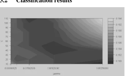
Figure 1: Contour plot of the classification error landscape resulting from a grid search over a range of values of {2-8, 2-7, 2-6, 2-5, 2-4} for the gamma parameter and a range of values of {10,

20, …, 110} for the C parameter on Wikipedia data.

Figure 2: Contour plot of the classification error landscape resulting from a grid search over a range of values of {2-8, 2-7, 2-6, …2-2} for the gamma parameter and a range of values of {1,

10, 20, 30, …110} for the C parameter on BioScope data.

Table 2: The performance of our system corresponding to the best parameter values. The performance is denoted in terms of true positives (TP), false positives (FP), false negatives (FN), precision (P),

recall (R) and F-score (F) .

the reference labels were made available, we also did tests with our system using the other two optimal settings for parameter values.

The optimal classification results on the Wikipedia dataset were obtained for a gamma value equal to 0.0625 and for a C value equal to 10, corresponding to a cross validation classification error of 17.94%. The model performances corresponding to these best parameter values are provided in Table 2. The P, R, F-score values provided in Table 2 are directly comparable to P, R, F-score values given in Table 1 since exactly the same datasets were used during the evaluation.

The SVM approach we adopted shows highly competitive empirical results for weasel detection on the Wikipedia test dataset in the sense that our system was ranked as the first in the CoNLL shared task. However, the baseline algorithm described in Section 2 proves to be rather difficult to beat given its F-score performance of 59% on the Wikipedia test data. This provides motivation to consider other refinements of our system. In particular, we believe that it might be possible to improve the recall of our system by enriching the list of input features using a lexical ontology in order to extract synonyms for verbs, adjectives and adverbs occurring in the current hedge cue list.

Figure 2 exemplifies the SVM classification results obtained during parameter tuning on BioScope training data. The optimal classification results on the BioScope dataset were obtained for gamma equal to 0.0625 and C equal to 110, corresponding to a cross validation classification error of 3.73%. The model performance corresponding to the best parameter settings is provided in Table 2. Our system obtained an F-score of 0.78 on the BioScope test dataset while the best ranked system in the CoNLL shared task obtained an F-score of 0.86. In order to identify the weaknesses of our system in this domain, in Subsection 3.2 we will furnish the intermediate results we obtained on the CoNLL training set.

The system is platform independent. We ran the experiments under Windows on a Pentium 4, 3.2GHz with 3GB RAM. The run times necessary for training/testing on the whole training/test dataset are provided in Table 2.

Table 3 shows the approximate intervals of time required for running SVM parameter tuning via grid search on the entire CoNLL training datasets.

Dataset Range of values Run

time

Wikipedia training data

{2-8,2-7, …2-1} for gamma;

{10, 20, …110} for

C

13 hours

BioScope training data

{2-8,2-7, …2-2} for gamma;

{10, 20, …110} for C

4 hours

Table 3 : Approximate run times for parameter tuning via 10-fold cross validation

3.3 Intermediate results

In the following we discuss the results obtained when the system was trained on approximately 80% of the CoNLL training corpus and the remaining 20% was used for testing. The 80% of the training corpus was also used to extract the list of hedge cues that were considered as input features for the SVM machine learning system.

The BioScope training corpus provided in CoNLL shared task framework contains 11871 sentences from scientific abstracts and 2670 sentences from scientific full articles.

In a first experiment, we only used sentences from scientific abstracts for training and testing: we randomly selected 9871 sentences for training and the remaining 2000 sentences were used for testing. The results thus obtained are shown in Table 4 on the second line of the table.

Dataset TP FP FN P R F Run Time

Table 4: Performances when considering separately the dataset containing abstracts only and the dataset containing articles from BioScope corpus. The SVM classifier was trained with gamma = 1 and c=10. Approximately 80% of the CoNLL train corpus was used for training and 20% of the train

corpus was held out for testing.

Second, we used only the available 2670 sentences from scientific full articles. We randomly split this small dataset into a training set of 2170 sentences and test set of 500 sentences.

Third, we used the entire set of 14541 sentences (composing scientific abstracts and full articles) for training and testing: we randomly selected 11541 sentences for training and the remaining 3000 sentences were used for testing. The results obtained in this experiment are shown in Table 4 on the fourth line.

We observe from Table 3 a difference of 10% between the F-score obtained on the dataset containing abstracts and the F-score obtained on the dataset containing full articles. This difference in accuracy might simply be due to the fact that the available abstracts training dataset is approximately 5 times larger than the full articles training dataset. In order to check whether this difference in accuracy is only attributable to the small size of the full articles dataset, we further analyze the learning curve of SVM on the abstracts dataset.

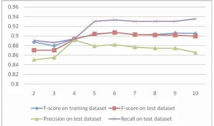
To measure the learning curve, we randomly selected from the abstracts dataset 2000 sentences for testing. We divided the remaining sentences into 10 parts, we used two parts for training, then we increased the size of the training dataset by one part incrementally. We show the results obtained in Figure 3. The x-axis shows the number of sentences used for training divided by 1000. We observe that the F-score on the test dataset changed only slightly when more than 4/10 of the training data (i.e. more than 4800 sentences) were used for training. We also observe that using 2 folds for training (i.e. approximately 2000 sentences) gives an F-score of around 87% on the held-out test data. Therefore, using a similar amount of training data for BioScope abstracts as used for BioScope full articles, we still have a difference of 8%

between the F-score values obtained. That is, our system is more efficient on abstracts than on full articles.

Figure 3: The performance of our system when we used for training various percentages of the BioScope training dataset composed of abstracts

only.

4 Conclusions

Our empirical results show that our approach captures informative patterns for hedge detection through the intermedium of a simple low-level feature set.

Our approach has several attractive theoretical and practical properties. Given that the system formulation is based on the max-margin framework underlying SVMs, we can easily incorporate other kernels that induce a feature space that might better separate the data. Furthermore, SVM parameter tuning and the process of building the feature vector matrix, which are the most time and resource consuming, can be easily integrated in a distributed environment considering either cluster-based computing or a GRID technology (Wegener et al., 2007).

From a practical point of view, the key aspects of our proposed system are its simplicity and flexibility. Additional syntactic and semantic

SVM Baseline

Dataset content #sentences

used for training

#sentences used for

test P R F P R F

Abstracts only 9871 2000 0.85 0.94 0.90 0.49 0.97 0.65 Full articles only 2170 500 0.72 0.87 0.79 0.46 0.91 0.61

Abstracts and full articles

based features can easily be added to the SVM input. Also, the simple architecture facilitates the system’s integration in an information retrieval system.

5 Future work

The probabilistic discriminative model we have explored appeared to be well suited to tackle the problem of weasel detection. This provides motivation to consider other refinements of our system, by incorporating syntactic or semantic information. In particular, we believe that the recall score of our system can be improved by identifying a list of new potential hedge cues using a lexical ontology.

References

Rong-En Fan, Pai-Hsuen Chen, and Chih-Jen Lin. 2005. Working set selection using the second order information for training SVM. Journal of Machine Learning Research, 6: 1889-918.

Richárd Farkas, Veronika Vincze, György Móra, János Csirik, and György Szarvas. 2010. The CoNLL-2010 Shared Task: Learning to Detect Hedges and their Scope in Natural Language Text.

In Proceedings of the Fourteenth Conference

on Computational Natural Language Learning (CoNLL-2010): Shared Task, pages 1–12.

Christiane Fellbaum. 1998. WordNet: An Electronic Lexical Database. MIT Press, Cambridge, MA.

Viola Ganter, and Michael Strube. 2009. Finding hedges by chasing weasels: Hedge detection using Wikipedia tags and shallow linguistic features. In Proceedings of joint conference of the 47th Annual Meeting of the ACL-IJCNLP.

Halil Kilicoglu, and Sabine Bergler. 2008. Recognizing Speculative Language in Biomedical Research Articles: A Linguistically Motivated Perspective. In Proceedings of Current Trends in Biomedical Natural Language Processing (BioNLP), Columbus, Ohio, USA.

Marc Light, Xin Ying Qiu, and Padmini Srinivasan. 2004. The Language of Bioscience: Facts, Speculations, and Statements in between. In Proceedings of the HLT BioLINK.

Chrysanne Di Marco, and Robert E. Mercer. 2004. Hedging in Scientific Articles as a Means of Classifying Citations. In Proceedings of Working Notes of AAAI Spring Symposium on Exploring Attitude and Affect in Text: Theories and Applications, Stanford University.

Alexa T. McCray, Suresh Srinivasan, and Allen C. Browne. 1994. Lexical methods for managing variation in biomedical terminologies. In Proceedings of the 18th Annual Symposium on Computer Applications in Medical Care.

Ben Medlock. 2008. Exploring hedge identification in biomedical literature. Journal of Biomedical Informatics, 41:636-54.

Ben Medlock, and Ted Briscoe. 2007. Weakly Supervised Learning for Hedge Classification in Scientific Literature. In Proceedings of the 45th Annual Meeting of the Association of Computational Linguistics.

Robert E.Mercer, Chrysanne Di Marco, and Frederick Kroon. 2004. The frequency of hedging cues in citation contexts in scientific writing. In Proceedings of the Canadian Society for the

Computational Studies of Intelligence

(CSCSI), London, Ontario.

György Móra, Richárd Farkas, György Szarvas, and Zsolt Molnár. 2009. Exploring ways beyond the simple supervised learning approach for biological event extraction. In Proceedings of the BioNLP 2009 Workshop Companion Volume for Shared Task.

Roser Morante, and Walter Daelemans. 2009a. Learning the scope of hedge cues in biomedical texts. In Proceedings of the BioNLP 2009 Workshop, Boulder, Colorado. Association for Computational Linguistics.

Roser Morante, and Walter Daelemans. 2009b. Learning the scope of hedge cues in biomedical texts. In Proceedings of the Workshop on BioNLP.

György Szarvas. 2008. Hedge classification in biomedical texts with a weakly supervised selection of keywords. In Proceedings of the ACL-08: HLT.

Vladimir N. Vapnik. 1998. Statistical learning theory. Wiley, New York.

Veronika Vincze, György Szarvas, Richárd Farkas, György Móra, and János Csirik. 2008. The BioScope corpus: biomedical texts annotated for uncertainty, negation and their scopes. BMC Bioinformatics, 9.