The Effects of Data Size and Frequency Range
on Distributional Semantic Models
Magnus Sahlgren Gavagai and SICS Slussplan 9, Box 1263 111 30 Stockholm, 164 29 Kista
Sweden
mange@[gavagai|sics].se
Alessandro Lenci University of Pisa via Santa Maria 36
56126 Pisa Italy
Abstract
This paper investigates the effects of data size and frequency range on distributional seman-tic models. We compare the performance of a number of representative models for several test settings over data of varying sizes, and over test items of various frequency. Our re-sults show that neural network-based models underperform when the data is small, and that the most reliable model over data of varying sizes and frequency ranges is the inverted fac-torized model.
1 Introduction
Distributional Semantic Models (DSMs) have be-come a staple in natural language processing. The various parameters of DSMs — e.g. size of con-text windows, weighting schemes, dimensionality reduction techniques, and similarity measures — have been thoroughly studied (Weeds et al., 2004; Sahlgren, 2006; Riordan and Jones, 2011; Bulli-naria and Levy, 2012; Levy et al., 2015), and are now well understood. The impact of various pro-cessing models — matrix-based models, neural net-works, and hashing methods — have also enjoyed considerable attention lately, with at times conflict-ing conclusions (Baroni et al., 2014; Levy et al., 2015; Schnabel et al., 2015; ¨Osterlund et al., 2015; Sahlgren et al., 2016). The consensus interpretation of such experiments seems to be that the choice of processing model is less important than the parame-terization of the models, since the various processing models all result in more or less equivalent DSMs (provided that the parameterization is comparable).
One of the least researched aspects of DSMs is the effect on the various models of data size and frequency range of the target items. The only pre-vious work in this direction that we are aware of is Asr et al. (2016), who report that on small data (the CHILDES corpus), simple matrix-based mod-els outperform neural network-based ones. Unfor-tunately, Asr et al. do not include any experiments using the same models applied to bigger data, mak-ing it difficult to compare their results with previous studies, since implementational details and parame-terization will be different.
There is thus still a need for a consistent and fair comparison of the performance of various DSMs when applied to data of varying sizes. In this pa-per, we seek an answer to the question:which DSM should we opt for if we only have access to lim-ited amounts of data?We are also interested in the related question: which DSM should we opt for if our target items are infrequent? The latter ques-tion is particularly crucial, since one of the major as-sets of DSMs is their applicability to create seman-tic representations for ever-expanding vocabularies from text feeds, in which new words may continu-ously appear in the low-frequency ranges.
In the next section, we introduce the contend-ing DSMs and the general experiment setup, before turning to the experiments and our interpretation of the results. We conclude with some general advice.
2 Distributional Semantic Models
One could classify DSMs in many different ways, such as the type of context and the method to build distributional vectors. Since our main goal here is
to gain an understanding of the effect of data size and frequency range on the various models, we fo-cus primarily on the differences in processing mod-els, hence the following typology of DSMs.
Explicit matrix models
We here include what could be referred to as ex-plicitmodels, in which each vector dimension cor-responds to a specific context (Levy and Goldberg, 2014). The baseline model is a simple co-occurrence matrixF (in the following referred to asCOfor
Co-Occurrence). We also include the model that results from applying Positive Pointwise Mutual Informa-tion (PPMI) to the co-occurrence matrix.PPMIis
de-fined as simply discarding any negative values of the PMI, computed as:
PMI(a, b) = logfab×T
fafb (1)
wherefab is the co-occurrence count of wordaand
word b,fa andfb are the individual frequencies of
the words, and T is the number of tokens in the
data.1
Factorized matrix models
This type of model applies an additional factor-ization of the weighted co-occurrence counts. We here include two variants of applying Singular Value Decomposition (SVD) to the PPMI-weighting
co-occurrence matrix; one version that discards all but the first couple of hundred latent dimensions (TSVD
fortruncatedSVD), and one version that instead re-movesthe first couple of hundred latent dimensions (ISVDforinvertedSVD). SVD is defined in the
stan-dard way:
F =UΣVT (2)
where U holds the eigenvectors of F, Σ holds the
eigenvalues, andV ∈U(w)is a unitary matrix
map-ping the original basis ofFinto its eigenbasis. Since V is redundant due to invariance under unitary
trans-formations, we can represent the factorization ofFˆ
in its most compact formFˆ ≡UΣ.
1We also experimented withsmoothedPPMI, which raises the context counts to the power ofαand normalizes them (Levy
et al., 2015), thereby countering the tendency of mutual infor-mation to favor infrequent events:f(b) = P#(b)α
b#(b)α, but it did not lead to any consistent improvements compared to PPMI.
Hashing models
A different approach to reduce the dimensionality of DSMs is to use a hashing method such as Random Indexing (RI) (Kanerva et al., 2000), which
accumu-lates distributional vectorsd(a)~ in an online fashion:
~
d(a)←d(ai)+~ c
X
j=−c,j6=0
w(x(i+j))πj~r(x(i+j)) (3)
wherecis the extension of the context window,w(b)
is a weight that quantifies the importance of context termb,2 ~rd(b) is asparse random index vectorthat
acts as a fingerprint of context termb, andπjis a
per-mutation that rotates the random index vectors one step to the left or right, depending on the position of the context items within the context windows, thus enabling the model to take word order into account (Sahlgren et al., 2008).
Neural network models
There are many variations of DSMs that use neural networks as processing model, ranging from simple recurrent networks (Elman, 1990) to more complex deep architectures (Collobert and Weston, 2008). The incomparably most popular neural network model is the one implemented in theword2vec li-brary, which uses the softmax for predictingbgiven
a(Mikolov et al., 2013):
p(b|a) = P exp(~b·~a) b0∈Cexp(~b0·~a)
(4)
whereCis the set of context words, and~band~aare
the vector representations for the context and target words, respectively. We include two versions of this general model; Continuous Bag of Words (CBOW)
that predicts a word based on the context, and Skip-Gram Negative Sampling (SGNS) that predicts the
context based on the current word.
3 Experiment setup
Since our main focus in this paper is the perfor-mance of the above-mentioned DSMs on data of
2We usew(b) = e−λ·f(Vb) wheref(b)is the frequency of context itemb,V is the total number of unique context items
varying sizes, we use one big corpus as starting point, and split the data into bins of varying sizes. We opt for the ukWaC corpus (Ferraresi et al., 2008), which comprises some 1.6 billion words after to-kenization and lemmatization. We produce sub-corpora by taking the first 1 million, 10 million, 100 million, and 1 billion words.
Since the co-occurrence matrix built from the 1 billion-word ukWaC sample is very big (more than 4,000,000 × 4,000,000), we prune the co-occurrence matrix to 50,000 dimensions before the factorization step by simply removing infrequent context items.3 As comparison, we use 200
di-mensions for TSVD, 2,800 (3,000-200) dimensions
forISVD, 2,000 dimensions forRI, and 200
dimen-sions for CBOWand SGNS. These dimensionalities
have been reported to perform well for the respec-tive models (Landauer and Dumais, 1997; Sahlgren et al., 2008; Mikolov et al., 2013; ¨Osterlund et al., 2015). All DSMs use the same parameters as far as possible with a narrow context window of±2words,
which has been shown to produce good results in se-mantic tasks (Sahlgren, 2006; Bullinaria and Levy, 2012).
We use five standard benchmark tests in these experiments; two multiple-choice vocabulary tests (the TOEFL synonyms and the ESL synonyms), and three similarity/relatedness rating benchmarks (SimLex-999 (SL) (Hill et al., 2015), MEN (Bruni et al., 2014), and Stanford Rare Words (RW) (Luong et al., 2013)). The vocabulary tests measure the syn-onym relation, while the similarity rating tests mea-sure a broader notion of semantic similarity (SL and RW) or relatedness (MEN).4The results for the
vo-cabulary tests are given in accuracy (i.e., percentage of correct answers), while the results for the similar-ity tests are given in Spearman rank correlation.
4 Comparison by data size
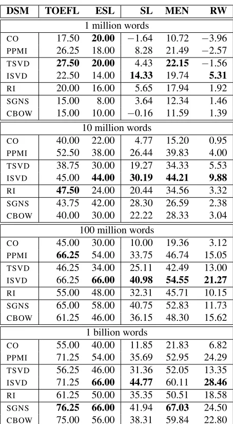
Table 1 summarizes the results over the different test settings. The most notable aspect of these results
3Such drastic reduction has a negative effect on the perfor-mance of the factorized methods for the 1 billion word data, but unfortunately is necessary for computational reasons.
4It is likely that the results on the similarity tests could be improved by using a wider context window, but such improve-ment would probably be consistent across all models, and is thus outside the scope of this paper.
DSM TOEFL ESL SL MEN RW
1 million words
CO 17.50 20.00 −1.64 10.72 −3.96 PPMI 26.25 18.00 8.28 21.49 −2.57
TSVD 27.50 20.00 4.43 22.15 −1.56
ISVD 22.50 14.00 14.33 19.74 5.31 RI 20.00 16.00 5.65 17.94 1.92 SGNS 15.00 8.00 3.64 12.34 1.46 CBOW 15.00 10.00 −0.16 11.59 1.39
10 million words
CO 40.00 22.00 4.77 15.20 0.95 PPMI 52.50 38.00 26.44 39.83 4.00 TSVD 38.75 30.00 19.27 34.33 5.53 ISVD 45.00 44.00 30.19 44.21 9.88
RI 47.50 24.00 20.44 34.56 3.32
SGNS 43.75 42.00 28.30 26.59 2.38 CBOW 40.00 30.00 22.22 28.33 3.04
100 million words
CO 45.00 30.00 10.00 19.36 3.12
PPMI 66.25 54.00 33.75 46.74 15.05
TSVD 46.25 34.00 25.11 42.49 13.00 ISVD 66.25 66.00 40.98 54.55 21.27 RI 55.00 48.00 32.31 45.71 10.15 SGNS 65.00 58.00 40.75 52.83 11.73 CBOW 61.25 46.00 36.15 48.30 15.62
1 billion words
CO 55.00 40.00 11.85 21.83 6.82 PPMI 71.25 54.00 35.69 52.95 24.29 TSVD 56.25 46.00 31.36 52.05 13.35 ISVD 71.25 66.00 44.77 60.11 28.46 RI 61.25 50.00 35.35 50.51 18.58
SGNS 76.25 66.00 41.94 67.03 24.50
[image:3.612.313.540.54.467.2]CBOW 75.00 56.00 38.31 59.84 22.80
Table 1:Results for DSMs trained on data of varying sizes.
is that the neural networks models do not produce competitive results for the smaller data, which cor-roborates the results by Asr et al. (2016). The best results for the smallest data are produced by the fac-torized models, with both TSVD andISVD
produc-ing top scores in different test settproduc-ings. It should be noted, however, that even the top scores for the smallest data set are substandard; only two models (PPMIandTSVD) manage to beat the random
base-line of 25% for the TOEFL tests, and none of the models manage to beat the random baseline for the ESL test.
The ISVD model produces consistently good
mil-0 20 40 60 80 100
1M 10M 100M 1G
,
[image:4.612.77.292.62.215.2]CO PMI TSVD ISVD RI SGNS CBOW
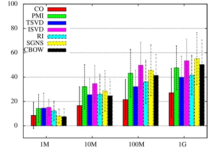
Figure 1:Average results and standard deviation over all tests.
lion and 100 million-word data, and is competitive with SGNS on the 1 billion word data. Figure 1
shows the average results and their standard devi-ations over all test settings.5 It is obvious that there
are no huge differences between the various models, with the exception of the baselineCOmodel, which
consistently underperforms. TheTSVDandRI
mod-els have comparable performance across the differ-ent data sizes, which is systematically lower than the
PPMI model. The ISVD model is the most
consis-tently good model, with the neural network-based models steadily improving as data becomes bigger.
Looking at the different datasets, SL and RW are the hardest ones for all the models. In the case of SL, this confirms the results in (Hill et al., 2015), and might be due to the general bias of DSMs to-wards semantic relatedness, rather than genuine se-mantic similarity, as represented in SL. The substan-dard performance on RW might instead be due to the low frequency of the target items. It is interesting to note that these are benchmark tests in which neural models perform the worst even when trained on the largest data.
5 Comparison by frequency range
In order to investigate how each model handles dif-ferent frequency ranges, we split the test items into three different classes that contain about a third of the frequency mass of the test items each. This
5Although rank correlation is not directly comparable with accuracy, they are both bounded between zero and one, which means we can take the average to get an idea about overall per-formance.
split was produced by collecting all test items into a common vocabulary, and then sorting this vo-cabulary by its frequency in the ukWaC 1 billion-word corpus. We split the vocabulary into 3 equally large parts; the HIGH range with frequencies rang-ing from 3,515,086 (“do”) to 16,830 (“organism”), the MEDIUM range with frequencies ranging be-tween 16,795 (“desirable”) and 729 (“prickly”), and the LOW range with frequencies ranging between 728 (“boardwalk”) to hapax legomenon. We then split each individual test into these three ranges, de-pending on the frequencies of the test items. Test pairs were included in a given frequency class if and only if both the target and its relatum occur in the frequency range for that class. For the constituent words in the test item that belong to different fre-quency ranges, which is the most common case, we use a separate MIXED class. The resulting four classes contain 1,387 items for the HIGH range, 656 items for the MEDIUM range, 350 items for the LOW range, and 3,458 items for the MIXED range.6
Table 2 (next side) shows the average results over the different frequency ranges for the various DSMs trained on the 1 billion-word ukWaC data. We also include the highest and lowest individual test scores (signified by↑and↓), in order to get an idea about the consistency of the results. As can be seen in the table, the most consistent model isISVD, which
produces the best results in both the MEDIUM and MIXED frequency ranges. The neural net-work modelsSGNSandCBOW produce the best
re-sults in the HIGH and LOW range, respectively, with CBOW clearly outperforming SGNSin the
lat-ter case. The major difference between these mod-els is that CBOW predicts a word based on a
con-text, whileSGNSpredicts a context based on a word.
Clearly, the former approach is more beneficial for low-frequent items.
The PPMI, TSVD and RI models perform
simi-larly across the frequency ranges, with RI
produc-ing somewhat lower results in the MEDIUM range, andTSVDproducing somewhat lower results in the
LOW range. The CO model underperforms in all
frequency ranges. Worth noting is the fact that all models that are based on an explicit matrix (i.e.CO,
DSM HIGH MEDIUM LOW MIXED CO 32.61 (↑62.5,↓04.6) 35.77 (↑66.6,↓21.2) 12.57 (↑35.7,↓00.0) 27.14 (↑56.6,↓07.9) PPMI 55.51 (↑75.3,↓28.0) 57.83 (↑88.8,↓18.7) 25.84 (↑50.0,↓00.0) 47.73 (↑83.3,↓27.1)
TSVD 50.52 (↑70.9,↓23.2) 54.75 (↑77.9,↓24.1) 17.85 (↑50.0,↓00.0) 41.08 (↑56.6,↓19.6)
ISVD 63.31 (↑87.5,↓36.5) 69.25(↑88.8,↓46.3) 10.94 (↑16.0,↓00.0) 57.24(↑83.3,↓33.0)
RI 53.11 (↑62.5,↓30.1) 48.02 (↑72.2,↓20.4) 23.29 (↑39.0,↓00.0) 46.39 (↑66.6,↓21.0)
SGNS 68.81(↑87.5,↓36.4) 62.00 (↑83.3,↓27.4) 18.76 (↑42.8,↓00.0) 56.93 (↑83.3,↓30.2)
CBOW 62.73 (↑81.2,↓31.9) 59.50 (↑83.3,↓32.4) 27.13(↑78.5,↓00.0) 52.21 (↑76.6,↓25.9)
Table 2:Average results for DSMs over four different frequency ranges for the items in the TOEFL, ESL, SL, MEN, and RW tests. All DSMs are trained on the 1 billion words data.
PPMI,TSVDandISVD) produce better results in the
MEDIUM range than in the HIGH range.
The arguably most interesting results are in the LOW range. Unsurprisingly, there is a gen-eral and significant drop in performance for low frequency items, but with interesting differences among the various models. As already mentioned, the CBOW model produces the best results, closely
followed by PPMI andRI. It is noteworthy that the
low-dimensional embeddings of the CBOW model
only gives a modest improvement over the high-dimensional explicit vectors ofPPMI. The worst
re-sults are produced by theISVDmodel, which scores
even lower than the baseline COmodel. This might
be explained by the fact that ISVD removes the
la-tent dimensions with largest variance, which are ar-guably the most important dimensions for very low-frequent items. Increasing the number of latent di-mensions with high variance in theISVDmodel
im-proves the results in the LOW range (16.59 when removing only the top 100 dimensions).
6 Conclusion
Our experiments confirm the results of Asr et al. (2016), who show that neural network-based models are suboptimal to use for smaller amounts of data. On the other hand, our results also show that none of the standard DSMs work well in situations with small data. It might be an interesting novel re-search direction to investigate how to design DSMs that are applicable to small-data scenarios.
Our results demonstrate that the inverted factor-ized model (ISVD) produces the most robust results
over data of varying sizes, and across several dif-ferent test settings. We interpret this finding as
fur-ther corroborating the results of Bullinaria and Levy (2012), and ¨Osterlund et al. (2015), with the con-clusion that the inverted factorized model is a robust competitive alternative to the widely usedSGNSand CBOWneural network-based models.
We have also investigated the performance of the various models on test items in different frequency ranges, and our results in these experiments demon-strate that all tested models perform optimally in the medium-to-high frequency ranges. Interestingly, all models based on explicit count matrices (CO, PPMI, TSVDandISVD) produce somewhat better results for
items of medium frequency than for items of high frequency. The neural network-based models and
ISVD, on the other hand, produce the best results for
high-frequent items.
None of the tested models perform optimally for frequent items. The best results for low-frequent test items in our experiments were pro-duced using theCBOWmodel, the PPMImodel and
the RI model, all of which uses weighted context
items without any explicit factorization. By contrast, theISVDmodel underperforms significantly for the
low-frequent items, which we suggest is an effect of removing latent dimensions with high variance.
This interpretation suggests that it might be inter-esting to investigatehybrid modelsthat use different processing models — or at least different parame-terizations — for different frequency ranges, and for different data sizes. We leave this as a suggestion for future research.
7 Acknowledgements
References
Fatemeh Asr, Jon Willits, and Michael Jones. 2016. Comparing predictive and co-occurrence based mod-els of lexical semantics trained on child-directed speech. InProceedings of CogSci.
Marco Baroni, Georgiana Dinu, and Germ´an Kruszewski. 2014. Don’t count, predict! a systematic compari-son of context-counting vs. context-predicting seman-tic vectors. InProceedings of ACL, pages 238–247. Elia Bruni, Nam Khanh Tran, and Marco Baroni. 2014.
Multimodal distributional semantics. Journal of Arti-ficial Intelligence Research, 49(1):1–47, January. John Bullinaria and Joseph P. Levy. 2012.
Extract-ing semantic representations from word co-occurrence statistics: stop-lists, stemming, and svd. Behavior Re-search Methods, 44:890–907.
Ronan Collobert and Jason Weston. 2008. A unified ar-chitecture for natural language processing: Deep neu-ral networks with multitask learning. InProceedings of ICML, pages 160–167.
Jeffrey L. Elman. 1990. Finding structure in time. Cog-nitive Science, 14:179–211.
Adriano Ferraresi, Eros Zanchetta, Marco Baroni, and Silvia Bernardini. 2008. Introducing and evaluating ukwac, a very large web-derived corpus of english.
Proceedings of WAC-4, pages 47–54.
Felix Hill, Roi Reichart, and Anna Korhonen. 2015. Simlex-999: Evaluating semantic models with (gen-uine) similarity estimation. Computational Linguis-tics, 41(4):665–695.
Pentti Kanerva, Jan Kristofersson, and Anders Holst. 2000. Random indexing of text samples for latent se-mantic analysis. InProceedings of CogSci, page 1036. Thomas K Landauer and Susan T. Dumais. 1997. A so-lution to platos problem: The latent semantic analysis theory of acquisition, induction, and representation of knowledge. Psychological Review, 104(2):211–240. Omer Levy and Yoav Goldberg. 2014. Linguistic
regu-larities in sparse and explicit word representations. In
Proceedings of CoNLL, pages 171–180.
Omer Levy, Yoav Goldberg, and Ido Dagan. 2015. Im-proving distributional similarity with lessons learned from word embeddings. Transactions of the Associa-tion for ComputaAssocia-tional Linguistics, 3:211–225. Minh-Thang Luong, Richard Socher, and Christopher D.
Manning. 2013. Better word representations with re-cursive neural networks for morphology. In Proceed-ings of CoNLL, pages 104–113.
Tomas Mikolov, Ilya Sutskever, Kai Chen, Greg S. Cor-rado, and Jeff Dean. 2013. Distributed representations of words and phrases and their compositionality. In
Proceedings of NIPS, pages 3111–3119.
Arvid ¨Osterlund, David ¨Odling, and Magnus Sahlgren. 2015. Factorization of latent variables in distributional semantic models. In Proceedings of EMNLP, pages 227–231.
Brian Riordan and Michael N. Jones. 2011. Redun-dancy in perceptual and linguistic experience: Com-paring feature-based and distributional models of se-mantic representation. Topics in Cognitive Science, 3(2):303–345.
Magnus Sahlgren, Anders Holst, and Pentti Kanerva. 2008. Permutations as a means to encode order in word space. InProceedings of CogSci, pages 1300– 1305.
Magnus Sahlgren, Amaru Cuba Gyllensten, Fredrik Espinoza, Ola Hamfors, Anders Holst, Jussi Karl-gren, Fredrik Olsson, Per Persson, and Akshay Viswanathan. 2016. The Gavagai Living Lexicon. In
Proceedings of LREC.
Magnus Sahlgren. 2006. The Word-Space Model. Phd thesis, Stockholm University.
Tobias Schnabel, Igor Labutov, David Mimno, and Thorsten Joachims. 2015. Evaluation methods for unsupervised word embeddings. In Proceedings of EMNLP, pages 298–307.