Forecasting Exchange Rate Volatility with High Frequency Data: Is the Euro Different?

Forecasting Exchange Rate Volatility with

High Frequency Data: Is the Euro Different?

Georgios Chortareas*

John Nankervis**

and

Ying Jiang***

This is a preliminary draft

Please do not quote without the authors’ permission

March 2006

Abstract

This paper focuses on forecasting volatility of high frequency Euro exchange rates. Four 15 minute frequency Euro exchange rate series, including Euro/CHF, Euro/GBP, Euro/JPY and Euro/USD, are used to test the forecast performance of six models, including both traditional time series volatility models and the realized volatility model. Besides the normally used regression test and accuracy test, an equal accuracy test, the HLN-DM test, and a superior predictive ability test are also employed in the out-of-sample forecast evaluation. The FIGARCH model is found to be superior in almost all exchange rate series. Although the widely preferred ARFIMA model shows better performance than the traditional daily volatility models, generally speaking, it cannot surpass the FIGARCH model and the intraday GARCH model. Furthermore, the SVX model does not significantly outperform the SV model in the accuracy test, which contradicts the results of some earlier research. The paper confirms the advantage of using high frequency data and modelling the long memory factor. It also analyses the characteristics of Euro exchange rates and compares the test results with the conclusions drawn by previous studies.

JEL classification: F31, C22

* (Corresponding author) Department of Accounting, Finance and Management, University of Essex, Wivenhoe Park, Colchester, CO4 3SQ, UK, Phone: 44-(0) 1206 874250. Email:

gchort@essex.ac.uk

** Department of Accounting, Finance and Management, University of Essex, Wivenhoe Park, Colchester, CO4 3SQ, UK, Phone: 44-(0) 1206 873973. Email: jcnank@essex.ac.uk

*** Department of Accounting, Finance and Management, University of Essex, Wivenhoe Park, Colchester, CO4 3SQ, UK. Email: jyianga@essex.ac.uk,

1

1. Introduction

For many years, the volatility forecast of the financial market and asset prices has been a focus for researchers, because of its importance for policy making, as well as investment analysis, derivative securities pricing and risk management. It is considered as a ‘barometer for the vulnerability of financial markets and the economy’ (Poon and Granger 2003). Besides some studies focusing on the application of volatility, up to 2002, there were at least 93 published or working papers studying modelling and forecasting volatility (Poon and Granger 2003), and this paper also falls into this category. The purpose of this paper is to evaluate the volatility forecast performance of various models for high frequency Euro exchange rates.

In recent years, using high frequency data has been the main focus of volatility forecasting. Before the research of Anderson et al. (1998a), which used intraday returns to calculate the measure for volatility forecasting, studies had normally concentrated on using daily returns to forecast volatility and daily squared returns as the measure of “true volatility”. However, as noted by Anderson et al.(1998a), daily squared returns are very noisy measure since they are calculated from daily closing prices and is impossible to reflect price fluctuations during the day. High frequency data, which carry more information of the daytime transactions, can significantly improve the accuracy in volatility forecasting. Thus more and more studies begin to use high frequency data, not only as a volatility measure, but directly in model estimation and forecasting as well. The examples include using the long memory ARFIMA model to model and forecast realized volatility, extending the daily model by including an intraday information term, and modelling standard volatility models on intraday returns directly. The comparison of these methods is set out in many studies, such as those of Martens (2001), Martens and Zein (2002), Hol and Koopman(2002), Andersen, Bollerslev, Diebold and Labys (ABDL thereafter) (2003) and others. These studies also confirm the advantages of using high frequency data. Although there have been plenty of studies on comparing volatility forecasting performance among models, there have not been, to the author’s knowledge, any studies based on high frequency Euro exchange rates. Therefore, choosing seldom studied data to compare the existing arguments is the first contribution of this study. Among various financial asset markets, the exchange rate market is the largest one in the world in terms of thetrading volume. Daily foreign exchange turnover can exceed 1.5 trillion American dollars (Source: Bank of International Settlements). Because dealers are widely spread in different time zones, unlike stock markets, the currency exchange market is open 24 hours a day. Therefore, it is also the most liquid market in the world, and the price is less likely to be affected by outside elements, such as the behaviour of individual traders or companies. Published studies and working papers on foreign exchange markets include but are not limited to West and Cho(1995), Anderson and Bollerslev(1998a), ABDL (1999,2000,2003), Martens (2001), Vilasuso(2002) and Jones (2003).

Since its introduction in 1999, the Euro has played an increasingly important role in global monetary markets. The Euro quickly established itself as the second most widely used international currency after the US dollar, ahead of the Japanese yen (Source:

2

European Central Bank). However, many of these studies focusing on the exchange rate volatility forecasting use USD exchange rates, mainly USD/JPY, USD/DEM or USD versus other important currencies, while few studies focus on high frequency Euro exchange rate volatility forecasting. Therefore, by choosing high frequency Euro exchange rates as the focus of the study, we may achieve different conclusions from those using other market data.

To carry out the study, both traditional time series volatility models and the realized volatility model are used and compared by evaluating their out-of-sample forecast performance. The traditional time series volatility models considered include the GARCH model, stochastic volatility (SV) model, stochastic volatilitywith exogenous

variables (SVX) model, and the long-memory FIGARCH model. The realized

volatility model is the long memory ARFIMA model. The GARCH model will be estimated by both intraday returns and daily returns. The inclusion of the daily GARCH model, the SV model and the SVX model is done so as to evaluate any possible advantage of using high frequency data.

The intraday GARCH model and the FIGARCH model are estimated by 15 minute frequency intraday returns to consider whether the traditional time series model can fit high frequency applications. Some studies have applied intraday returns to standard volatility models, including Beltratti and Morana (1999), Martens (2001), Rahman and Ang(2002), and Marlik(2005). However, most of these studies use a relatively small number of observations and lower frequencies. Using a large number of high frequency intraday returns with standard volatility models is the second contribution of this study. Moreover, the intraday GARCH and the FIGARCH models are compared with the recent proposed realized volatility model, the ARFIMA model, which has not been previously done in the literature. In addition, the comparison of two kinds of long memory models in high frequency application, i.e., the FIGARCH model and the ARFIMA model, has received little attention by the other studies. Filling this gap can be considered the third contribution.

Besides the contributions mentioned above, by comparing the GARCH model with

theFIGARCH model, the paper also contributes to a better understanding of whether modelling the long memory property in a high frequency volatility process can improve the forecast performance for short forecasting horizons, which is not commonly seen in previous studies.

To evaluate the out-of-sample forecast performance, various tests have been performed in this study. In addition to the normally used regression test and accuracy test, to further study the inferences from the accuracy test, an equal accuracy test, the adjusted Diebold-Mariano(1995) test (Harvey, Leybourne and Newbold, 1997) and the superior predictive ability test (Hansen, 2005) are also employed. The results of these tests show that the FIGARCH model has outperformed the ARFIMA model after the deseasonalisation of raw returns, and the intraday GARCH also shows good performance. Such a result is rather surprising, since it has not been reported in previous research. Furthermore, the paper on the one hand confirms that using high frequency data can substantially enhance the forecast performance, and on the other hand, finds that when we consider the long memory factor, i.e. comparing the FIGARCH and GARCH models, the results show the benefits of modelling the long memory. The paper also shows that daily GARCH performs slightly better than the

3

SV and SVX models in terms of the accuracy test, while this result again contradicts earlier findings that the SVX model can outperform the original daily volatility model.

The remainder of the paper is arranged as follows: Chapter 2 introduces some main findings and current arguments in volatility forecasting literature related to this paper. Chapter 3 focuses on the data and methodology used in this paper. Chapter 4 discusses the parameter estimation results and the fitness for each model. Chapter 5 compares the out-of-sample forecast performance of the models according to the results from different tests. The conclusions are given in Chapter 6.

2. Literature Review

Given the importance of volatility, numerous studies related to volatility forecasting have appeared. The review will mainly concentrate on those studies related to the application of high frequency data. Studies reviewed here can be classified into four groups:

Studies focusing on realized volatility start with Andersen and Bollerslev (1998a) whoconstructs the realized volatility by summing the squared intraday returns and the first paper that proposes the realized volatility to be a volatility measure. The paper shows the dramatic improvement of the forecast performance of a daily GARCH model by using the new volatility measure. This study can be regarded as the seminal paper on using high frequency data in volatility forecasting.

A number of further studies by the same authors focus further on the forecasting of realized volatility and its properties. ABDL (1999) first recommends without application, the ARFIMA model for forecasting realized volatility after studying the properties of the distributions of realized volatility and realized covariance. ABDL (2000) supports the argument that realized volatility is an efficient estimator of integrated volatility by showing the empirical results that the returns standardized by realized volatility are nearly normally distributed. The main contribution of ABDL (2001) is that it recognizes that realized volatility can benefit forecasting if it is directly modelled by a parametric model rather than simply used as an evaluation of other models’ forecasting behaviour. The findings of the above studies constitute the theoretical base of directly using realized volatility in volatility forecasting. Following this idea, ABDL (2003) proposes a long memory Gaussian vector autoregression process (VAR) to model and forecast realized volatility and the value at risk. This paper gives us strong empirical evidence that the VAR-RV model provides superior performance to other candidate models.

A second strand in the literature considers the merits of alternative models and compares daily with high frequency data. Many papers focus on testing the benefits of using high frequency data and comparing different methods for forecasting volatility, including the realized volatility method mentioned above, the traditional time series model and the option implied method.

Martens (2001) compares daily volatility forecasts constructed from multiple volatility forecasts of intraday intervals, with a daily model and a daily model extended by intraday information. It finds that the higher the intraday frequency is

4

used, the better are the out-of-sample daily volatility forecasts. The daily model, including intraday information, has similar performance to the method that models intraday returns directly. Martens and Zein (2002) provides the evidence that using high frequency data can improve both the accuracy of measurement and the performance of forecasting. It also shows that the long memory model contributes to its improvement as well. Hol and Koopman (2002) adopt the high frequency return series of the S&P100 stock index and use two kinds of models: realized volatility models and daily time-varying volatility models to compare their predictive power. The results of the out-of-sample evaluation show that the ARFIMA model estimated by realized volatility gives the most accurate forecast. Pong, Shackleton and Taylor (2004) compares among option implied volatility and the forecasts obtained from the short memory model--ARMA, the long memory model---ARFIMA, and the daily GARCH model. It finds that the most accurate historical forecasts come from the use of high frequency returns, not from a long memory specification.

All of these studies confirm that using high frequency data can improve the volatility forecast performance. They also reach a consensus that the forecast from high frequency data can outperform the option implied volatility, which is regarded as the superior volatility forecast in the literature in the daily case. Furthermore, for the studies using realized volatility, they all show that this method is superior to the traditional time series models.

The question that naturally emerges is whether the standard models still valid and a pate of papers attempt to address this issue. As more and more evidence supports the realized volatility method, which models realized volatility directly, another question is raised that whether traditional time series models can capture the unique properties of high frequency data and fit the intraday return series. However, no consensus has been achieved yet. For example, Rahman and Ang (2002) shows that intraday volatility can be best described by a standard GARCH(1,1) model, while Jones (2003) suggests that the standard time series models cannot capture the intraday exchange rate return generating process at the frequencies higher than 24 hours by using the simulation method.

Finally, another set of studies considers the properties of high frequency data for specific markets. The inferences mentioned above related to high frequency data are all based on analysing the properties of developed financial markets. Dacorogna et al.(2001) demonstrates some stylized properties for high frequency exchange market returns, such as the non-normal distribution, first order negative autocorrelation, increasing fat tail when the frequency increases, the seasonality and so on. Meanwhile, there are some other studies trying to answer the question whether these stylized properties also apply to other markets. Kayahan and Stengos (2002) use the Istanbul Stock Exchange and Barbosa (2002) studies the Brazil inter bank FX market. They both confirm that the high frequency data of the special markets they choose have similar features to the stylized properties concluded from developed markets.

Based on the findings of the current literature, examining whether these inferences are also valid in Euro exchange rates is the main focus of this paper. Therefore, the aim of this study is to analyse the properties of the high frequency Euro exchange rates, choose some popularly discussed methods in the literature and evaluate their forecast ability.

5

3. Data and Methodology

3.1 Data and their properties

The original data sets are 5-minute interval spot foreign exchange prices of Euro/CHF, Euro/GBP, Euro/JPY and Euro/USD provided by Olsen and Associates.

These currencies are chosen because they are the major ones in terms of the trading volume, which account for over 85% of all foreign exchange transactions. In addition, these non-USD currency pairs are all direct trading currencies, and thus it avoids using cross rates, which are calculated from the USD exchange rates.

The original data set is from January 1st, 2000 to October 31st, 2004 for a total of 509,472 observations for each exchange rate series. The starting year of 2000, rather than 1999 is chosen to exclude the unstable period of the Euro due to its initial introduction.

Although the data are available in 5-minute intervals, the 15-minute frequency is used in this study. Many researchers assume that the higher the frequency, the more accurate forecast. However, it has also been argued that extremely high frequency does not necessarily produce the best result, because of market microstructure effects (ABDL, 1999). There is no consensus on what is the optimal interval to fit in order to balance the accuracy and microstructure disturbances. In practice, 5-minute and 30-minute intervals are commonly used. To balance between the cost of huge computation time of 5-minute data and relatively less accuracy of 30-minute intervals, the 15 minute interval is used in this research and the price series are constructed from an initial grid of 5-minute prices.

The currency exchange market is open 24 hours a day, 7 days a week. However, very small trading volumes can be observed on weekends and holidays. Similar to Anderson and Bolleslev(1998a), weekend returns from Friday 21:05 GMT to Sunday 21:00 GMT are removed from the sample. The returns of January 1, December 25, 26 as well as Good Friday and Easter Monday are also removed.

The return series r_t is obtained by:

1 ln ln − ₋ = _{t t} t p p r (1)

where p_t is the spot price at time t.

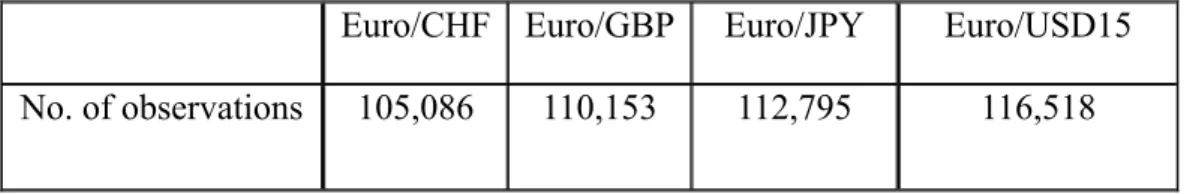
After the deletion of the missing values in the raw price set, the final numbers of sample observations in the return series are shown in Table 1 and the actual plots of each return series are shown in Graph 1.

Table 2 shows the summary statistics of the distribution of raw returns for each exchange rate series. From the figures we can learn that the 15-minute returns of Euro exchange rates have similar characteristics to those stylized properties of high frequency financial time series returns documented in the literature. For example, the values of kurtosis are far greater than the normal distribution indicating fat tailed distributions. Three of the Euro exchange rate returns series are slightly skewed, while for Euro/USD, the skewness is as high as 0.966. The means of the series concerned

6

here, like other financial returns, are all approximately zero.

Dacorogna et al.(2001) discuss in detail the stylized properties of high frequency data in foreign exchange markets. One of these properties is about kurtosis. It not only confirms the well known large value of kurtosis for the return series, but also discusses the relationship between the value of kurtosis and the frequency of returns. In this study, we confirm their findings about this relationship by comparing the kurtosis of three different frequency returns. Table 3 shows the kurtosis of 5-minute, 15-minute and 30-minute returns for each exchange rate series. The figures demonstrate the kurtosis increases as the time frequency increases, i.e. the highest frequency—the 5-minute return has the largest kurtosis.

Another stylized property of the high frequency return documented in Dacorogna et al(2001), as well as many other studies is the negative first order autocorrelation in returns. Graph 2 shows the ACF of each 15-minute Euro exchange rate returns. Large negative autocorrelations in the first lag can be observed. The autocorrelations after the first lag are rather small. This phenomenon is caused by the bounce between bid and ask prices, which is a market microstructure effect.

However, when we consider the Box-Pierce test statistics up to 36 lags, the large values indicate the hypothesis that these return series are white noise is rejected. Lobato, Nankervis and Savin (2001) propose a modified Q test, which allows the statistical dependence of the series to be considered; the hypothesis is still rejected, using their adjusted Q-test for our series. The autocorrelation after the first order in raw returns is not reported in other studies on USD exchange rates for example, ABDL (2003), or Dacorogna et al(2001). However, the serial dependence in raw returns is found in some high frequency stock markets (Andersen et al., 2001 and Rahman and Ang, 2002), which means that the property of Euro exchange rates may differ from that of USD exchange rates, while it does not contradict the stylized properties of high frequency data.

In addition, there is another important property of the data, i.e., seasonality of intraday volatility. Graph 3 shows the ACF of absolute returns of 4 exchange rate series. The apparent U shape seasonality can be observed for every 24 hours. For the 15-minute return series, there are 96 observations per 24 hours, so the pattern can be observed at every 96 lags, which strongly indicates the seasonality with a period of one day. The autocorrelation is highest at the beginning and the end of the 24 hour intervals, and is lowest at the middle. This property has also been confirmed by other studies, such as Anderson and Bollerslev (1997), Barbosa (2002), and Dacorogna et al (2001), etc. According to Dacorogna et al(2001), this phenomenon is due to the overlap of opening hours of the three major foreign exchange markets in the world, the American, European and Asian markets. When both American and European markets open, the autocorrelations are relatively large. From the graph we can also see that the persistence of autocorrelation in absolute returns dies out very slowly, indicating the long memory property in the volatility process.

In summary, the 15-minute Euro exchange rate series used in this study have stylized properties similar to those of other high frequency financial returns reported in the literature. They are all fat tailed, slightly skewed (except Euro/USD) and zero mean. There is a positive correlation between the kurtosis and the frequency of the returns.

7

They share not only negative first order autocorrelation, but also significant ‘spurious’ autocorrelation after the first lag in raw returns. Most importantly, they have strong seasonality in intraday volatility.

3.2 Models and Estimation

Six models will be used in the study: a realized volatility model ARFIMA model, intraday GARCH and FIGARCH models, a daily GARCH model, a stochastic volatility model and an extended stochastic volatility model. It is widely considered that the long memory process exists in the volatility series, and the ARFIMA model can capture well this property in daily realized volatility. However, it is still interesting to test whether there is any difference between modelling realized volatility directly (ARFIMA) and embedding the long memory in a GARCH type model (FIGARCH). A GARCH (1,1) model is chosen because studies show in most of the cases, other volatility models can’t beat a simple GARCH(1,1) model by using daily data. Therefore, its performance in high frequency cases is an interesting topic. In addition, not much work has been done in comparing thestandard GARCH model with its long memory counterparts, especially for intradayEuro exchange rate returns. For example, Vilasuso (2002) and Lux and Kaizoji(2004) compare GARCH and FIGARCH in volatility forecasting, but they use daily data. Zumbach(2002) uses one-hour returns with USD exchange rates. The stochastic volatility model is extended by an intraday information term in order to evaluate whether high frequency returns help daily volatility forecasting.

The intraday returns show strong seasonality in 24 hour intervals, which has been demonstrated in the previous section. As noted by, among others, Anderson and Bollerslev(1997) and Martens, Chang and Taylor(2002), the estimation of traditional time series models, e.g., GARCH type models, will be corrupted by intraday seasonality. Therefore, the deseasonalised filtered returns will be used to estimate traditional time series models rather than directly use intraday returns. The filtered return is defined as the nth _{intraday return divided by an estimated seasonality term.}

R~t= ( 1... ) , , N n S R n d n d = (2) where R_d,n is the nth intraday return on day d, while Sd,nis the corresponding

seasonality term, supposing there are N intraday periods.

n d

S _, is estimated by the method proposed by Taylor and Xu(1997), which simply

averages the squared returns for each intraday period: ) .... 1 ( 1 ˆ 1 2 , 2 N n R D s D d n d n =

∑

Graph 4 shows the ACF of absolute filtered returns for each exchange rate series. It can be observed that by this method, seasonality is well extracted and the U shape pattern is almost removed for all series. The filtered returns will be used to estimate

theintraday GARCH model and the FIGARCH model.

8

returns will be fit into the GARCH (1,1) model. The model is estimated by the

maximum likelihood method using the Eviews package. For the intraday GARCH

model, an MA (1) process is used in the mean equation in order to filter the serial correlation in the intraday return series caused by the microstructure effect. The MA (1)-GARCH(1,1) model is defined by:

) , 0 ( ~ | , ~ 1 1 t t t t t t D h R =ε +θε ₋ ε Ω₋ 1 1 2 1 1 + − + = ₋ t t h h t β ε α ω (4) The t-distribution is chosen as the error distribution in order to capture the fat tail often occurring in standardized GARCH innovations. Daily returns used to estimate the daily GARCH model are defined as the difference of logarithm prices at 12:00 pm GMT on that day and at 12:00 pm GMT on previous day, which will result in 1,237 daily return observations.

The FIGARCH model extends the variance equation of the standard GARCH model by including fractional differences to capture the long memory properties in volatility. Following Baillie, Cecen and Han(2000), we specify an MA(1)- FIGARCH(1,d,0) model in this study, which can be written as:

) , 0 ( ~ | , ~ 1 1 t t t t t t D h R =ε +θε ₋ ε Ω₋ 2 1 1 1 (1 (1 ) ) t d t t h L L h =ω+β ₋ + −β − − ε (5)

where d is the order of fractional integration, and L is the lag operator.

The FIGARCH model is estimated using the 15 minute returns data and one step ahead forecasts are produced. The model is estimated by the Quasi maximum likelihood method with Student-t error distribution using the G@CH package (Laurent, and Peters, 2005) written in the Ox language of Doornik (2001).

The ARFIMA (p,d,q) model (Granger and Joyeux,1980) for a series ytis defined

by t t d L y L L µ θ ε φ( )(1− ) ( − )= ( ) (6) where d is the order of fractional integration, and L is the lag

operator. P

PL

L

L φ φ

φ( )=1+ ₁ +_K+ is the AR polynomial component,

q qL L

L θ θ

θ( )=1+ 1 +K+ is the MA polynomial component and µ is the mean of

t

y .

According to ABDL (2003), ytis defined as logarithm daily realized volatility

log (σt). Depending on the sample spectrum of data, not all parameters of an

ARFIMA model can be identified from the data, especially in the case of realized volatility (Hol and Koopman, 2002). Therefore, empirically, many studies set a fixed d instead of estimating it. According to the specification of ABDL (2003), in this study d is fixed to 0.401 and the order of the model is set at (5,d,0).

In this paper, daily realized volatility is constructed by the 15-minute return series. In order to take account of the serial correlation in raw returns, an MA(1) filtered return is used. The following are all filtered returns.

The daily realized variance is defined by:

∑

9

where the variance of day t is equal to the sum of squared intraday returns. Consistent with the one day definition of the daily GARCH model, realized volatility is also calculated from the returns between 12:00 pm on day t-1 and 12:00 pm on day t. Therefore the ARFIMA (5, d, 0) model specified in this research is:

t t d L L σ µ ε θ( )(1− ) (log(ˆ )− )= (8) The model is estimated by the maximum likelihood method using the ARFIMA package (Doornik and Ooms, 2001) written in the Ox language of Doornik (2001). In the Stochastic Volatility model (Taylor,1994), volatility is modelled as an unobserved latent variable. It is argued that the SV model can capture the main empirical properties often observed in daily financial returns in a more appropriate way than GARCH type models (Broto and Ruiz, 2004). Therefore, the comparison of their performance in Euro exchange rate volatility forecasting is one of the interests of the study. In addition, the performance of the SV model and the SVX model has been evaluated by earlier studies on stock markets, such as Hol and Koopman (2002), and it will be useful to compare the results obtained in the case of the Euro exchange rates. A standard SV model is defined as:

) 1 , 0 ( ~ , ), exp( , ,... 1 ), 1 , 0 ( ~ , 1 2 * 2 NID h h h T t NID y t t t t t t t t t t η η σ φ σ σ ε ε σ η + = = = = − (9) where ytdenotes the return series and it is assumed that εt and ηtare uncorrelated.

The volatility process is the product of a squared scale parameter _σ*_{and the}

exponential of the stochastic processht.

Hol and Koopman (2000) specify a SV model with implied volatility as an explanatory variable in the variance equation, and this model is referred to as the SVX model. Following Hol and Koopman(2002), we use intraday returns as the explanatory variable instead of implied volatility in the SVX model. The mean and variance equations of the SVX model are identical to those of the standard SV model, while the ht process is specified as:

t t

t

t h L x

h =φ ₋₁+γ(1−φ ) ₋₁+σ_ηη (10)

where x_t−1 is the intraday information defined as the sum of 15 minute squared

intraday returns.

The parameters of the SV model will be estimated by the simulated maximum likelihood method using the importance sampling technique. It is carried out by a program written in the Ox language of Doornik (2001) using SsfPack by Koopman, Shephard and Doornik (1999). The program is downloaded from the webpage of ‘Analysis of Stochastic Volatility using SsfPack’, which is created by Koopman. 3.3 Forecasting

One hundred days are used to be theout-of-sample period for the forecast evaluation. The in-sample estimation period is from January 4th, 2000 to June 11th, 2004. For the ARFIMA model, SV model, SVX model and daily GARCH (1, 1) model, 1,137 daily returns are used for initial model estimation and the one-step-ahead daily volatility forecast is produced. This procedure is repeated 100 times in order to produce 100

10

daily volatility forecasts for out-of-sample evaluation. The ARFIMA model and daily GARCH (1, 1) are estimated recursively while for the SV models, the rolling window method is used according to the original downloaded program.

For the intraday GARCH (1, 1) and FIGARCH (1, d, 0) models, the initial estimation period is from 12:00 pm January 3rd, 2000 to 12:00 pm June 11th, 2004. By using recursive estimation, the next 15 minute ahead forecasts are produced. The number of forecasts may be different for each series, because the numbers of missing values in each return series are different. However, theoretically, 9,600 intraday variance forecasts should be produced if there is no missing value in the return series. Since the forecasts are based on deseasonalised filtered returns, the variance forecasts have to be transformed back to those from original returns by multiplying by the appropriate seasonal term_ˆ2 n s , i.e. 2 , 2 2 , ˆ ~ ˆ_{t fn} s_n σ_{t fn} σ = ∗ (11) where 2 , ~ fn t

σ is the 15-minute ahead variance forecast for deseasonalised filtered

returns, 2

n

s is estimated by the method mentioned in last section, and σˆ_t2_,fn is the

transformed forecast for original returns.

In accordance with the idea of realized volatility, the daily variance forecast is calculated by:

∑

σ is intraday variance forecasts during the day t and 2 ,

ˆ_{f t}

σ is daily variance forecast on day t. 100 daily variance forecasts can be obtained by summing the intraday variance forecasts.

Therefore, six series of forecasts are produced fromsix different models (to be exact: five different models and two different sample frequencies) and the forecast evaluation can be carried out based on them.

4 Evaluating Alternative Forecasts

4.1 True volatility measure

Because the true volatility is unobservable, a proxy will be used as the measure of volatility forecasts. According to Andersen and Bollerslev (1998a), realized volatility is an unbiased and more accurate proxy of true volatility than the popularly used daily squared returns. In this research, the realized volatility is constructed from 5-minute returns and used as the proxy of true volatility.

∑

r is thesquared intraday return and σrv2_,t is therealized variance on day t.

There is no universal standard forecast evaluation method to judge the forecast of models, and this study chose some popularly used methods in the literature.

11

4.2 Regression test-Predictive power test:

The basic idea of the regression test is that the true volatility is regressed on a constant and forecasted volatility in order to examine whether the forecasted value has explanatory power for the true volatility. In this essay we use realized volatility to be the proxy of true volatility, and the regression is as follows:

t t forecast t realized α βσ ε σ _,+1 = + ˆ _,+1 + (14) where _{σrealized,t+1} is realized volatility at time t+1, σˆ_forecast,t+1is the forecasted value for true volatility of time t+1 predicted at time t.

The R2 from the regression can be used for the assessment of the predictability of our models.

This approach is introduced by Mincer and Zarnowitz (1969) and is further studied by Hatanaka (1974). It has also been widely used in forecasting evaluation by many researchers, such as Pong, Shackleton, Taylor and Xu (2004), Martens, Chang and Taylor(2002), Anderson and Bollerslev (1998a), Balaban (1999), and ABDL (2003). This study will estimate 24 OLS regressions between actual volatility and forecasted volatility from 6 models with 4 exchange rates series each. A larger R2_{means that}

the true volatility can be better explained by the forecasted one in the equation and the model producing that forecast has more powerful forecast ability.

4.3 Heteroskedasticity Adjusted Root Mean Squared Error (HRMSE)-Accuracy test:

HRMSE belongs to the accuracy test, which compares the “true volatility” with the forecasted value and calculates the forecast error. Among various accuracy criteria, the mean error (ME), mean squared error (MSE), mean absolute error (MAE), root mean squared error (RMSE), mean absolute percentage error (MAPE), and heteroskedasticity adjusted root mean squared error (HRMSE) are most commonly used. However, there is no standard to decide which one is the best. In this study, in order to take account of heteroskedasticity in forecast errors, we chose HRMSE, which is also used by ABDL (1999), Martens and Zein (2002) and Hol and Koopman (2002).

The HRMSE is calculated by

2 1 ,, 1 1 , , ₎ ˆ ˆ 1 ( 1

_∑

4.4 Diebold-Mariano Test and HLN adjust DM test:

However, the model with a smaller forecast error does not mean it is significantly superior to other models. In other words, the difference between two forecasts might be insignificantly different from zero. Thus,Diebold and Mariano (1995) propose an “equal accuracy” test between two forecasting models.

12

Let g(•) be a specified loss function, and in our case, HRMSE. g (et₁) and g (et2) are

two forecast error series coming from two competing models. The loss differential is defined by d_t =g(e_t1)−g(e_t2). The null hypothesis of equal forecast accuracy isE[g(e_t1)]= E[g(e_t2)] or d_t=0. If the null is rejected, it indicates the model with the

smaller loss is significantly superior to the other model.

The procedure of the DM parametric test is as follows: let dtbe a loss differential

series with mean

∑

= = T t t d T d 1 1

. The DM test statistic is defined by

) ( ˆ _d V d DM =

where Vˆ(d) is the asymptotic variance of d . The estimator is calculated as

] ˆ 2 ˆ [ 1 ) ( ˆ 1 1 0

∑

∑

limit theory, the DM test statistics will have an asymptotic standard normal distribution under the null hypothesis.

However, it is argued that for finite samples, the normal distribution can be a very poor approximation, and the test statistics may be biased depending on the degree of serial correlation among forecast errors.

Harvey, Leybourne, and Newbold (1997) (HLN) suggest an adjusted DM test statistic that improves small-sample properties:

DM T T h h h T DM HLN _ = +1−2 + ( −1)/ (18)

where the test statistic is compared with the a Student-t-distribution with (T-1) degrees of freedom. Monte Carlo simulation confirms that the HLN_DM performs much better at all forecast horizons if the forecast errors are autocorrelated or have non-normal distributions (Harris and Sollis 2003).

4.5 Superior Predictive Ability Test (Hansen 2005)

In practice, the selection of the most accurate forecast is always among a set of

models. Unlike the DM test, which compares forecasts from only two competing

models, the superior predictive ability (SPA) test introduced by Hansen (2005) evaluates the performance of several alternative models. In addition, it assesses whether the same outcomes can be obtained from more than one sample by the use of a bootstrap procedure. In the SPA test, a benchmark model is selected and ‘the question of interest is whether any alternative forecast is better than the benchmark forecast’ (Hansen 2005).

13

loss function. In this study, the SPA test is taken by the SPA code written by Ox (Hansen, Kim and Lunde, 2003). In the code, two loss functions are predefined, which are the mean squared error (MSE) and mean absolute error (MAE). We chose both of them in order to compare the result with the HRMSE used in theDM test.

The intraday FIGARCH model is chosen as the benchmark model, since the empirical results discussed in next section show it produces the smallest HRMSE for all the

exchange rate series. Therefore, whether the FIGARCH model significantly

outperforms the alternative models by other criteria is our question of interest.

5.

Empirical Results for In-sample Estimation

All the parameter estimators for the realized volatility model, daily model and intraday model discussed below, are estimated by the first in-sample period returns. This is because the in-sample period is changing for every forecast step, and we only analyse the first estimation result as the example to explain the models’ fitness. We start with the results of the MA (1)-GARCH (1, 1) and MA(1)-FIGARCH(1,d,0) models. Table 4 shows the parameters of the intraday MA (1)-GARCH (1, 1), MA (1)-FIGARCH (1, d, 0), as well as daily GARCH (1, 1) models. Table 5 shows the residual test of three models for four exchange rate return series.

In Table 4, all MA (1) parameters in the mean equations are negative, which captures the first order negative autocorrelation in the returns. For the intraday GARCH (1, 1) model, all the parameters in the mean equations and variance equations are significant. The fact that α+β<1 shows the GARCH process is stationary. In most cases the sum is close to 1 indicating the persistence of volatility. The same situation also applies to the daily GARCH (1, 1). This evidence shows that the properties of 15 minute intraday returns can be well captured by the MA (1)-GARCH (1, 1) specification and the daily GARCH also fits the daily returns well. For the FIGARCH model, the long memory parameter d is significantly different from zero for all series, indicating that the long memory property in the volatility process has been captured. The value of d is around 0.2 for all cases, which is similar to the value estimated by Baillie, Cecen and Han (2000) that uses different exchange rate series and different frequencies. As mentioned in Baillie, Cecen and Han (2000), this phenomenon supports the argument of the ‘invariant’ property of the long memory parameter. However, for theEuro/CHF series, under the specification of FIGARCH (1, d, 0), the parameter β is not significant. The insignificant parameter β of Euro/CHF shows there are some distinguishable properties in the Euro/CHF series and the order (1, d, 0) is not appropriate for this series. We have tried different orders, such as (1,d,1) and (0,d,1), and found that (0,d,1) fits the data best, which indicates that the Euro/CHF return series is an ARCH process rather than GARCH process under a long memory specification. The fractional parameter d is also close to 0.2 and significant. Therefore the forecast on Euro/CHF volatility will be produced by a FIGARCH (0, d,1) model. The model fitness can also be checked by diagnostic tests on residuals. Table 5 shows the residual tests of the above mentioned models. The Q-test for the standardized

14

residual up to 50 lags shows the non-autocorrelation hypothesis is rejected for both intraday GARCH and FIGARCH models. In addition, for the intraday GARCH (1, 1) model, the Q-test for the squared standardized residual indicates that there are still serial correlations existing. However, for the FIGARCH model, the serial correlation in standardized squared returns is eliminated in most of the cases, except the Euro/GBP series. An ARCH-LM test rejects the hypothesis of no ARCH effect in the residual from the intraday GARCH model in any case, but it cannot reject the hypothesis for Euro/CHF from the FIGARCH model. In addition, although for the other 3 series, the p-values of the ARCH(10)-LM test for the FIGARCH model are less than 5%, the test statistics of FIGARCH are much less than those from the intraday GARCH model. This evidence indicates that the FIGARCH model can better capture the dependence and persistence in volatility than the GARCH model for the intraday case. While for daily cases, the results for the daily GARCH model show it successfully fits in the daily returns.

Nevertheless, the good in-sample model fitness does not necessarily lead to a superior out-of-sample forecast. To select a powerful prediction model, we should also consider the performance of out-of-sample forecasts.

The second specification that we use is an ARFIMA (5, d, 0) model. ABDL (2003) use a long memory VAR-RV to model logarithmic daily realized volatility and find that it has the best forecast for exchange rate volatility. In this study, an ARFIMA model is applied to 4 individual exchange rates. For the order of the model and parameter d, we follow ABDL (2003), i.e., ARFIMA (5, d, 0) with d=0.401.

In fact, before the decision of using the same specification as ABDL (2003), some alternative orders and an estimated d were also tried for comparison. However, the information criteria AIC preferred the order (5, d, 0) to other orders, such as (1, d, 1) and (1, d, 0). In addition, we also tried to estimate the parameter d for each series. For in-sample estimation, the decrease of AIC was trivial and most importantly, its out-of-sample performance was similar and slightly inferior to the fixed d case. Therefore, we keep the specification of ABDL (2003).

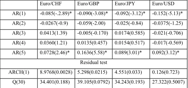
Table 6 shows the estimation result of ARFIMA models for each series. Interestingly, only the first and the fifth order autoregressive parameters are significant. Since the series under consideration is logarithmic volatility, the model fitness cannot be compared with GARCH-type models. Nevertheless, Table 6 also shows the residual test for the ARFIMA model. The Q-test on standardized residual indicates the ARFIMA model captures well the volatility dependency, but the ARCH-LM tests get low p-values, except for the Euro/USD series.

Moving to the typical Stochastic Volatility Model, Table 7 reports the log likelihood values and residual test results for the two models. It is interesting that all the log likelihood values from the SV model are larger than those from the corresponding SVX model that includes intraday information. This result is contrary to the findings of Hol and Koopman (2002) and Koopman, Jungbacker and Hol(2005), which report that the SVX model has higher log likelihood for the S&P 100 stock market. Nevertheless, the Q-test and the normality test on the residuals indicate both models fit the daily return series successfully for all cases.

15

6. Empirical results for out-of-sample forecast evaluation

6.1 The regression test

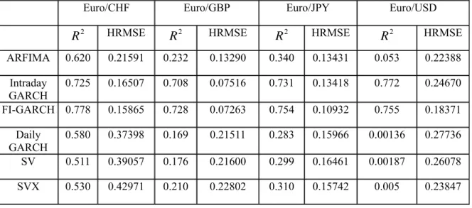
With regard to the result of the regression test, we can classify the 6 models into 3 categories according to their performance. The FIGARCH and Intraday GARCH lead the test, which provides us with enough surprises and interest; because the earlier literature has not shown that the traditional volatility model estimated by intraday returns can surpass the realized volatility model, ARFIMA model. From Table 8 we can see that in all series, the R2s from the regressions of intraday GARCH and FIGARCH exceed 70%, which means that most true volatility can be explained by the forecast. This result is far better than the second category model, ARFIMA. For

example, the R2 from the FIGARCH model is 25.5% higher than that from the

ARFIMA model for the Euro/CHF case, 263.8% for Euro/GBP, 121.76% for Euro/JPY and 1,324.5% for Euro/USD. If we further compare the two leading models, we can find the FIGARCH has a little bit more predictive ability than the intraday

GARCH in most cases, except the Euro/USD series. The R2 _{from FIGARCH is}

7.3% higher than intraday GARCH for Euro/CHF, 2.8% for Euro/GBP, and 3.0% for Euro/JPY. However, for the Euro/USD case, the R2 from intraday GARCH is 2.2% higher than that from the FIGARCH model.

If we exclude intraday GARCH and FIGARCH models, then the result is similar to most previous findings, i.e., the realized volatility model ARFIMA is preferred, rather than the traditional daily volatility models. Although the SVX model has already included intraday information, which is proved, in other studies, to be an efficient method to forecast volatility, it still cannot catch up with the ARFIMA model in any series. Also from Table 8, we can see their differences from the following figures:

the R2 of the ARFIMA model is 17.9% higher than that of the SVX model for

Euro/CHF, 11.5% for Euro/GBP, 11.1% for Euro/JPY and 960.0% for Euro/USD. The traditional volatility models, daily GARCH, SV and SVX, belong to the third category. Just as expected, their performance is in no way satisfactory, especially for the Euro/USD series. The R2s are extremely low in this series and the highest figure, which is from the SVX model, is only 0.5%. Although the results are better in the other three series, they still lag far behind the models in categories one and two. According to Martens and Zein (2002), Jones (2003), Hol and Koopman(2002), Koopman, Jungbacker and Hol(2005) and some others, including intraday information can improve the performance of traditional daily volatility models. In our study, if we compare the SVX model and SV model, the higher R2s values from the SVX model for all the series indicate that true volatility can be explained more by the forecast from the SVX model, which is consistent with previous studies. When we compare the SV and daily GARCH models, the R2s from the SV model are higher than those from daily GARCH in most of the cases, except the Euro/CHF series. This result is consistent with some earlier studies, such as Yu (2002) and Lopez (2001). Actually, the comparison results between the GARCH model and SV model in the literature are mixed. For example, Dunis Laws and Chauvin (2000) reports that the SV model performs worst among daily volatility models.

16

From the foregoing results we can draw an inference that the intraday models perform best, the realized volatility model (ARFIMA) is in the middle tier, while the traditional daily volatility models cannot compete in most cases.

6.2 HRMSE

According to the results of the HRMSE, we can also divide the 6 models into 3 same categories. Similar to the results of the regression test, the intraday GARCH model and FIGARCH model produce smaller forecast errors in most of the cases, except for the Euro/USD series, where the HRMSE from the ARFIMA model is smaller than that from the intraday GARCH model and ranks second among the 6 models. Nevertheless, the FIGARCH model for the Euro/USD series still has the smallest HRMSE comparing with others and therefore for all the series, the FIGARCH model ranks first in the accuracy test. This result together with the result of the regression test shows that the FIGARCH model has the greatest predictive power and produces the most accurate forecast. In some cases, the intraday GARCH model or the ARFIMA model is close to the FIGARCH model, which will be further verified by the equal accuracy test, while their differences with the daily volatility models are rather large. For

example, the FIGARCH model produces 57.5% lower HRMSE than the daily

GARCH model for Euro/CHF, 66.2% for Euro/GBP, 31.5% for Euro/JPY, and 33.8% for Euro/USD.

Although generally speaking, the HRMSE has similar results to the regression tests, when we look to the 3 daily volatility models, their results are not always compatible. Most previous studies have shown that the SVX has better performance than the SV model, which is also confirmed by the regression test in this study. However, such an advantage for SVX does not appear in the HRMSE case. For Euro/CHF and Euro/GBP, the HRMSE from the SVX model is much larger than those from the SV model. For the Euro/JPY series, the SVX model has a smaller HRMSE than the SV model, but the difference is negligible.

In addition, if we compare the SV model with the daily GARCH model, the result of HRMSE is not in line with that of the R2 test either. For Euro/GBP and Euro/JPY series, the HRMSE of the SV model is not as good as daily GARCH, which is contrary to the result of the R2 test. Such a result can usually be found in volatility forecast literature, because different forecast evaluation methods may prefer different models. It is a puzzle that researchers select their own models in accordance with their preferred methods.

In summary, the regression and accuracy tests in this study have not only confirmed some arguments proposed by other researchers, but also given different results. On the one hand, the realized volatility model ARFIMA has a better performance than traditional daily volatility models, which agrees with many pervious studies. On the other hand, however, we believe that the FIGARCH and intraday GARCH models have even more outstanding predictive ability than the ARFIMA model, which has not been, at least to the author’s knowledge, reported in the literature. Furthermore, the results of the 3 daily volatility models are mixed and different models may be chosen according to different evaluation methods.

17

6.3 The HLN-DM test

In order to further evaluate the accuracy of forecasts among the models, an equal accuracy test of HRMSE is also adopted in this study.

Table 9 shows the statistics of the HLN-DM test of 5 pairs of models for 4 exchange rate series. The test compares the significance of the difference between HRMSEs from two competing models pair by pair. According to the order given by the HRMSE, the HLN-DM test will be used 5 times for each series. First, the two smallest HRMSEs are chosen to calculate test statistics and then the inferior one will be compared with the next superior HRMSE among the rest. The test statistics for 5 pairs’ comparison results are reported in Table 9.

From Table 8 we can see the orders of HRMSE values for Euro/CHF and Euro/GBP series are same. Therefore these two series will be first discussed together. The first two columns of Table 9 show the test statistics of 5 pairs of models for the two series. We can see that the differences between the FIGARCH and intraday GARCHmodels are insignificantly different from zero. The intraday GARCH is significantly superior to the ARFIMA model with large statistics, and the differences between the SV model and SVX model are also significant for the two series. However, there is no significant difference between the daily GARCH model and the SV model for Euro/GBP.

For the Euro/JPY series, the HLM-DM test shows different results. Only two pairs, FIGARCH v.s. intraday GARCH and ARFIMA v.s. SVX, have significant statistics, and the differences of all the other pairs are insignificant.

The Euro/USD series also shows a surprising result. First of all, the FIGARCH model is significantly superior to the ARFIMA model, while the differences between the ARFIMA model and intraday GARCH model, intraday GARCH model and SVX model are insignificant. Among the daily volatility models, the SVX model is significantly superior to the SV model, and the later is also significantly better than the daily GARCH model.

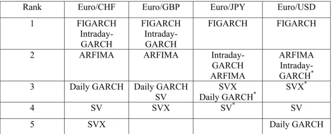
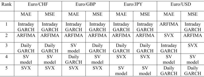
Table 10 shows the rank given by the HLM-DM test for 4 exchange rate series. Models in the same rank mean the HRMSEs from them are statistically equal, while the model in the second line inside the grid has a relatively larger HRMSE. From the table we can see that the results of the first 2 ranks are similar to those of the regression test. The FIGARCH model always performs best for all the cases. The intraday GARCH model is superior to the ARFIMA model in two cases and not different with the ARFIMA in the other two. This result shows that the ARFIMA model can have similar forecast ability to the intraday GARCH model, but it never surpasses the latter or the FIGARCH model. In addition, daily volatility models cannot surpass the intraday models or the realized volatility model.

The results of daily volatility models are rather mixed. The daily GARCH model surprisingly ranks the 3rd in 3 cases, although 2 of them share this rank with another equal accuracy model. This result again contradicts the regression test result that the SVX model performs best and the results of Hol and Koopman (2002) and Koopman, Jungbacker and Hol(2005) that the SVX model is superior to the daily GARCH model

18

in the accuracy test . It also brings an opposite result to the earlier studies that support the hypothesis that the SV model is superior to the daily GARCH model.

6.4 Superior Predictive Ability (SPA) test

Another more efficient method to check the significance of the superiority of models is the SPA test. The test will select 6 models among a large number of competing models, which are the most significant model, best model, models with a performance relative to 25% ,50%(median), and 75% of the benchmark model and the worst model. In this study, we only have 5 competing models besides the benchmark model, and therefore the result of the SPA test also shows the rank of 5 models at the same time. The benchmark model is the FIGARCH model, which is unanimously preferred by thethree tests discussed above.

Table 11 shows the result of the SPA test for each series by two evaluation criteria. It lists the model selection, sample loss, t-statistics and “p-values”. At the bottom of the panel for each series, the p-values of the SPA test are reported, which are in bold font and marked by yellow colour. The figures show that the null hypothesis that the FIGARCH model is not inferior to other models cannot be rejected for any case with the exception of Euro/CHF evaluated by the MSE. The MSE of intraday GARCH is smaller than that of the FIGARCH model for the Euro/CHF case. This is not surprising, because sometimes the result is sensitive to the evaluation method. However, according to the majority of the cases, we can conclude that generally speaking, the FIGARCH model cannot be surpassed by other models.

Table 12 summarises the rank given by the SPA test. The result is similar to the rank by HRMSE. In most of the cases, the intraday GARCH and ARFIMA models follow the FIGARCH model closely with a better performance by the intraday GARCH model. The three daily volatility models have mixed rankings, while the daily GARCH model gets more chances to rank ahead of the other two, which is consistent with the result of HRMSE. One surprising exception is that for the Euro/USD evaluated by MAE case, the SVX model, next to the ARFIMA model, has a smaller MAE even than the intraday GARCH model. However, if we look at the rank from MSE and HRMSE, the result above is not so surprising, since the SVX model also performs best among daily models in both criteria for the Euro/USD series. Therefore, we can conclude that the Euro/USD series prefers the SVX model to other daily models, and in some extreme cases it can outperform the intraday GARCH model.

6.5 Discussion of the out-of sample-performance of the tests

Combining the parameter estimation result from section 4 and the forecast evaluation result above, we get the following findings. First, the FIGARCH model not only fits the data better than the intraday GARCH model for in-sample estimation, but also shows superior forecast performance in almost all of the exchange rate series. The HLN-DM test further proves that such superiority to the intraday GARCH model is significant in two cases. With these advantages in both aspects, the FIGARCH model is selected as the most favourable model. This is the most important finding in this research, since the FIGARCH model has seldom been found as a powerful model in high frequency forecasting. The advantages of FIGARCH over the intraday GARCH model, with the only difference in the consideration of the long memory,

19

also confirm the FIGARCH model captures well the long memory characteristic of high frequency volatility and gains benefits from it for forecasting.

The widely preferred ARFIMA model cannot surpass the FIGARCH model or the intraday GARCH model. The good performance of the latter shows that, at least for our Euro exchange rates, the traditional daily volatility model can still be quite effective after the deseasonalisation of high frequency returns. Both being long memory models, the FIGARCH and ARFIMA models are different in the way of modelling the long memory properties in volatility. The test in this study shows that with the adoption of high frequency data, the long memory GARCH family model has clear advantages over the long memory realized volatility model.

The result that models using high frequency data have far better results than the daily volatility models proves that using high frequency data can effectively improve the forecast performance. Such a conclusion has also been drawn in many earlier studies and once again is confirmed by this study.

The SVX model not only has inferior model fitness to the SV model, but also gets poor forecast performance in terms of the forecast error. It only outperforms the SV model in two cases. Although the regression test shows that the SVX model is the best among the daily models, the accuracy test results contradict the results of the earlier studies that the daily model extended by intraday information should produce a more accurate forecast. However, for the Euro/USD exchange rates, the SVX model shows good performance, which is consistent with the earlier findings.

The in-sample estimation result of the daily GARCH model cannot be simply compared with the SV family models. However, its forecast performance shows in most of the cases, its forecast accuracy is better than, or at least equal to, theSV type models. The result of this study further confirms the mixture of comparison results between the GARCH and SV models in the literature. In addition, the accuracy and regression tests provide different outcomes. This reminds us to be aware that different evaluation methods may have different preferences.

Some seemingly surprising results from the Euro/USD series in fact are in line with the studies on USD exchange rates or other data. Such a coincidence may indicate that USD and Euro exchange rates might prefer different models. Therefore, it is difficult to have a general answer for the superiority of models, and the current conclusions are data sensitive. This is a difficult problem for volatility forecasters and explains why there are so many contradictory conclusions.

7. Conclusion

The main aim of this study is to forecast volatility of the euro exchange rates by using high frequency data. As a newly emerged important currency, the Euro has already shown great strength and huge potential in financial markets. However, current studies on currencies still concentrate on the USD and do not give due attention to the Euro. This study therefore fills a gap and achieves some different findings on model selection from those studies on USD exchange rates and stock markets.

20

model, daily volatility models estimated by intraday returns, daily volatility model extended by intraday information and simple daily volatility models. Four Euro exchange rate series were adopted, including Euro/CHF, Euro/GBP, Euro/JPY and Euro/USD. To explore new possibilities, the frequency of data was designed as the 15 minute interval, which is not popularly used.

After the various tests specified in previous chapters, we can draw the following conclusions. The most important finding of the study is that the FIGARCH model surpasses all of the other models selected and takes the lead in most of the out-of-sample evaluation tests. This result also surprises the author, because FIGARCH has seldom been regarded as a competitive model in high frequency application. From the author’s point of view, such success is due to its ability to capture, at the same time, both the long memory and volatility clustering properties, which are the two most important characteristics of volatility. Furthermore, the employment of high frequency data also helps FIGARCH to achieve substantial advantages over the daily volatility models. These combined factors may explain why FIGARCH can fare so well in the forecast competition. Meanwhile, the

shortcoming of applying the high frequency framework to the FIGARCH model is

also obvious, i.e., with current available packages and computer equipment, running FIGARCH in high frequency data is rather time consuming. Such a disadvantage will restrict the wide use of the model at the present stage.

Besides the FIGARCH model, the intraday GARCH model also performs fairly well in forecasting. This result breaks the prejudice that the traditional daily volatility model cannot fit the high frequency data framework. Many researchers in this field believe that the ARFIMA model is a highly effective one for high frequency data. However, after the deseasonalisation of the raw returns, the traditional GARCH family models can still adapt highly volatile intraday data and acquire even more satisfactory forecast results than the newly developed models. At a time when most volatility forecast studies use high frequency data, this result reminds us that the improvement of traditional models has equal importance to the development of all kinds of new models.

It is now a common practice for volatility forecasters to use high frequency data, because the strong evidence of improvement after its adoption has been proved in many articles. This study again demonstrates this point. The least difference of R2 in the regression test for high frequency and daily data is 6.8% and for the accuracy test, the smallest difference also reaches 6.3%. This article, like many others, provides a solid foundation for proving the contribution of high frequency data.

This study analyses the properties of Euro exchange rates and finds that they are similar to the stylized properties of high frequency data, which have been disclosed by some earlier studies on other foreign exchange rates or stock markets. This suggests that these properties are not subject to certain kinds of high frequency data, but most probably reflect the general feature that all such data share. Meanwhile, Euro exchange rates also possess some unique characteristics that are different from other rates, such as the USD. For example, there are autocorrelations in the Euro exchange rate raw returns. This difference possibly explains some unusual conclusions that have been drawn by this study.

21

In general, this study achieves some different conclusions and at the same time, confirms some earlier findings in the literature. These inferences might have some valuable influence on future volatility forecasting. Nevertheless, there are still many issues that need to be considered: First, the result of the study is based on the single regime model and does not take account of possible structural change in the volatility process. There is a reason for us to consider the regime-switching model, which might produce more satisfactory results by using time-varying parameter models in the series. Second, the advantage of the realized volatility model is its simplicity and less computation without losing the accuracy of the forecast. To fully tap the potential of the realized volatility model, more models need to be explored. Third, as mentioned before, although the FIGARCH model had the best performance in the test, the great amount of computation is an incentive to develop more powerful computation methods to meet the requirements of huge observations of high frequency data. Last but not the least, the Euro was introduced 6 years ago, and such a short period may not be enough to fully reflect the complexity of its fluctuations. As it matures, we may acquire more data for a longer sample period, and it will help us to make a more thorough investigation of it.

22

Appendix: Data Processing

The data set includes 5-minute interval price series of four exchange rates. It contains 509,472 observations and the period is from January 1st, 2000 to October 31st 2004. Different data series are computed from the raw data set in order to make the corresponding estimations and evaluations. The data is processed by following steps:

1. Create price series with different frequencies. The 15-minute, 30-minute and daily interval price series are created from the raw data set by deleting appropriate grids of prices. For example, for each hour, only the spot prices at minute 0, 15, 30, and 45 are kept in order to construct the 15-minute interval price series. The 30-minute series is used to compare the return kurtosis with those of the 5-minute and 15-minute series. The daily series is used for the estimation of the daily GARCH model and the SV models.

2. Create the 15-minute price series without weekend data. In this step, the prices from Friday 21:05 GMT to Sunday 21:00 GMT are removed from the series. 3. Deseasonalize 15-minute returns to estimate the intraday GARCH model and

the FIGARCH model. First, the return series are calculated by equation (1) and the missing values are removed from the series. Second, equations (2) and (3) are used to calculate deseasonalized returns for the estimation of intraday models. Therefore the forecasts from the intraday GARCH model and FIGARCH model are “deseasonalized forecasts”.

4. Transform the deseasonalized forecasts to those based on the raw returns. By using equation (11), the transformed intraday variance forecast series are obtained.

5. Calculate daily variance forecasts for intraday models. Based on the idea of realized volatility, the daily variance forecasts are obtained by equation (12), which sums the intraday variance forecasts for a day. The daily variance forecasts are the final forecasting result of intraday models that will be compared with those from other models.

6. Calculate two series of realized volatility. By using equation (7), the realized volatility series used for estimating the ARFIMA model and that used as the proxy of true volatility are created. The former one is constructed by 15-minute interval returns while the latter is by 5-minute interval returns.

For each exchange rate, there are totally 10 data series created for different purposes. Steps (1) and (2) are realized by Visual Basic Application in Excel. The rest steps are carried out by the codes written in Ox language.