Bacteria Biotope Relation Extraction via Lexical Chains and Dependency Graphs

158

Bacteria Biotope Relation Extraction via Lexical Chains

and Dependency Graphs

Wuti Xiong1, Fei Li2, Ming Cheng3, Hong Yu2, Donghong Ji1 1. School of Cyber Science and Engineering, Wuhan University, China

2. Department of Computer Science, UMass Lowell, USA 3. Department of Medical Information,

The First Affiliated Hospital of Zhengzhou University, China

[email protected],[email protected]

Abstract

In this article, we describe our approach for the Bacteria Biotopes relation extraction (BB-rel) subtask in the BioNLP Shared Task 2019. This task aims to promote the development of text mining systems that extract relationships between Microorganism, Habitat and Pheno-type entities. In this paper, we propose a novel approach for dependency graph construction based on lexical chains, so one dependency graph can represent one or multiple sentences. After that, we propose a neural network model which consists of the bidirectional long short-term memories and an attention graph convo-lution neural network to learn relation extrac-tion features from the graph. Our approach is able to extract both intra- and inter-sentence relations, and meanwhile utilize syntax infor-mation. The results show that our approach achieved the best F1 (66.3%) in the official evaluation participated by 7 teams.1

1 Introduction

The BioNLP Shared Task 2019 (Bossy et al.,

2019) is a continuation of the previous efforts or-ganized around the BioNLP Shared Task work-shop series (Kim et al.,2009,2011;N´edellec et al.,

2013;Del´eger et al., 2017). It aims to facilitate development and sharing of computational tasks of biomedical text mining and solutions to them. The Bacteria Biotope (BB) task is one of the six main tasks of the BioNLP Open Shared Tasks 2019. Three teams participated in the BB task when it was first organized in 2011. INRA Bib-liome (Ratkovic et al.,2011) achieved the best Fs-core of 45% with the Alvis system which used dic-tionary mapping, ontology inference and semantic analysis for NER, and co-occurrence-based rules for detecting relations between the entities. The 2013 BB task (Bossy et al.,2013) contained three

1_{Code: https://github.com/woodyXwt/BB19-rel}

Figure 1: Bacteria Biotopes relation examples. The Red, green and blue words denote Microorganism en-tities, Habitat entities and Phenotype entities respec-tively.

subtasks, the first one concerning recognition and normalization of bacteria and habitat entities, and the other two subtasks involving relation extrac-tion. Four teams participated in these tasks, with the UTurku TEES system (Bj¨orne and Salakoski,

2013) achieving the first places with F-scores of 42% and 14%. Compared to the 2013 BB task, the 2016 BB task contains more subtasks and its subtask2 only concerned relation extraction. The team VERSE (Lever and Jones, 2016) achieved the best F-scores of 55.8% in the subtask2.

Fig-ure1shows some examples for each relationship. In the BB-rel task, not all the relations occur be-tween two entities with the same sentence. In the preprocessing step, we found that there exist about one fourth of all relations whose argument enti-ties are located in different sentences. Therefore, we need to build a model that does not only con-sider the entity relationship within one sentence, but also beyond the sentence boundary.

A lexical chain (Morris and Hirst,1991) is a se-quence of words which are semantically-similar or related. These words are related sequentially in the text, defining the topic of the text seg-ment that they cover and establishing associations between sentences. Following this observation, some researchers have obtained success in many NLP tasks such as word sense induction(Tao et al.,

2014) , machine translation (Mascarell,2017) and text (Stokes et al., 2004) segmentation. In the BB-rel dataset, the sentences where inter-sentence relations occur usually express the same topic or have semantic associations each other. These fea-tures usually appear as some related words which can form lexical chains. Following this obser-vation, we propose a novel approach to build an inter-sentence dependency graph based on lexical chains.

In this paper, we propose a novel relation ex-traction method for the BB-rel task by incorpo-rating dependency graphs and lexical chains into the neural network. As shown in Figure1, sentence relations are usually expressed in inter-related sentences, and these sentences may con-tain semantically-related words which can form lexical chains. We utilize these lexical chains and dependency graphs to build an inter-sentence dependency graph for inter-sentence relation ex-traction. Specifically, we utilize word embed-ding to find the semantic relationships of words that occur in different sentences for building re-liable lexical chains. Then, we use the Stanford CoreNLP toolkit (Manning et al., 2014) to ob-tain sentence-level dependency and part-of-speech (POS) information, and build an inter-sentence de-pendency graph based on these information and lexical chains.

After that, we employ a neural network model which consists of the bidirectional long short-term memories and attention-guided graph convo-lutional neural networks to extract features from the inter-sentence dependency graph. The

fea-Train Dev

Lives In 715 395

Exhibits 281 138

Total relatonships 996 533

Intra-sentence relationships 885 467 Inter-sentence relationships 111 66

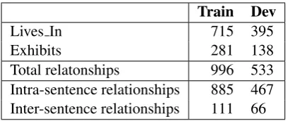
Table 1: BB-rel data statistics on the training and de-velopment set.

tures are fed into a multi-layer perceptron (MLP) to classify the relation between an entity pair.

Our approach has two advantages. First, it is ca-pable of extracting both intra-sentence and inter-sentence relations by connecting the dependency graphs of different sentences via lexical chains. Second, it is able to leverage syntax information. The results in the BB-rel task demonstrate the su-periority of our method. It achieves the highest F1-score, the second highest precision and recall in the official evaluation.

2 Method

In this section, we first introduce our strategy of relation candidate generation. Then, the approach for constructing lexical chains is described. After that, we will introduce how to build inter-sentence dependency graphs. Lastly, the architecture of our neural network model is described.

2.1 Relation Candidate Generation

In the BB-rel dataset, if all candidate pairs (bac-teria and habitat or phenotype) that occur in the document are enlisted as candidate training exam-ples, the positive and negative examples will be-come very unbalanced because most entity pairs located beyond one sentence do not have any re-lation. Based on our observations, most entity pairs spanning more than two sentences have no relations between them. Therefore, we consider all entity pairs that span within two sentences as the candidates to generate training examples. The statistics of our dataset are summarized in Table1.

2.2 Lexical Chain Construction

Figure 2: Process of lexical chain construction. Orange words denote nouns.Cis the set of lexical chains. The similarity here refers to the cosine similarity between word vectors. We set the threshold to 0.5.

automatically extracted lexical chains using statis-tical methods . Another approach (Li et al.,2017) is based on semantic word vectors. In this paper, we assume that lexical relationships can be cap-tured by calculating the similarity of their seman-tic vectors. To compute similarities, we use 200-dimensional pre-trained word vectors released by Pyysalo et al. (2013). Moreover, we only consider nouns for constructing the lexical chains since they usually contain relevant information.

Given a sentence, we first use the Stanford CoreNLP toolkit (Manning et al., 2014) to ob-tain POS tags for each word. Then we pick those words whose POS tags belonging to N= (NN,NNP,NNS)as candidates for chain construc-tion. We take one candidate at a time and check where it should be placed. Assuming thatCis the set of lexical chains, we add each candidatewtoC according to the following steps (Figure2):

• Step 1: each noun is treated as a candidate w. IfCis empty, we will create a new lexical chain in C and add the current candidate w into it.

• Step 2: for the current candidate w, we tra-verse all the lexical chains inCand compute the similarity between the last word of each lexical chain and the current candidatew. If the similarity surpasses a predefined thresh-old, the current candidatewwill be attached to the corresponding lexical chain.

• Step 3: if the current candidate wcannot be attached to any existing lexical chain, we will create a new lexical chain for it.

Figure 3: An example of the dependency graph and its corresponding adjacent matrix. If there is a dependency relation between the node i andj in the dependency graph, the value of the elementMijin the adjacent ma-trix is 1.

2.3 Dependency Graph Construction

In this section, we propose an approach to build an inter-sentence dependency graph by lexical chains. For an entity pair that occurs within the same sentence, we directly use their sentence de-pendency graph. If two entities occur in different sentences, we construct their dependency graph by lexical chains. We design two rules to build an inter-sentence graph. Here we define the follow-ing notations:Cis the set of lexical chains,Aand

Bare nouns belonging to sentences1and sentence s2, respectively.

• Rule 1: ifAandBexist in the same chain of

C, we will add an edge betweenAandB to build an inter-sentence dependency graph.

• Rule 2: ifAandBdo not appear in the same lexical chain, we will use the root nodes of two sentences to build the dependency inter-sentence graph.

Then we convert the dependency graph into an adjacency matrix. An example of such pro-cess is shown in Figure 3. Give a sequence

S = {s1, s2, ..., sn}, we considered its

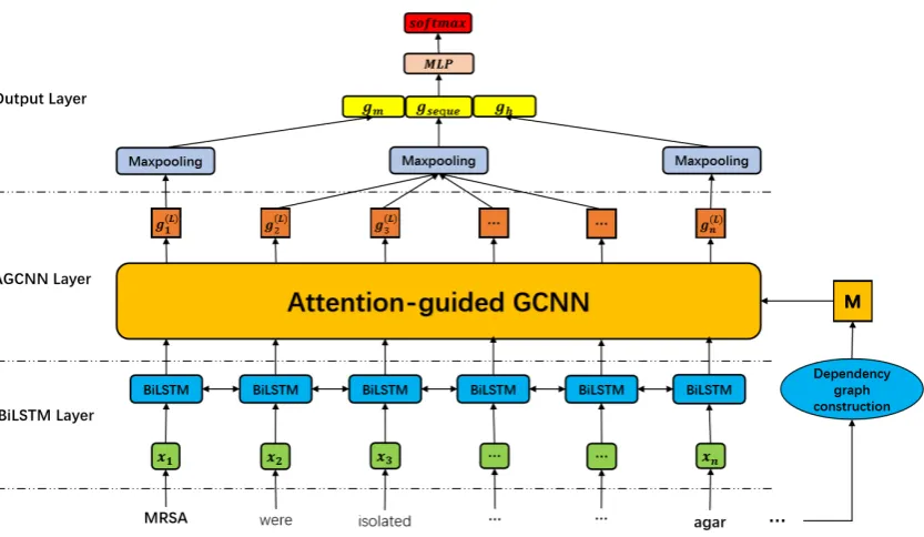
Figure 4: The architecture of our model. The input sentence is “MRSA were isolated by oxacillin screening agar” with a Microorganism entity “MRSA” and a Habitat entity “oxacillin screening agar”. M denotes the adjacency matrix.

2.4 Neural Network Model

2.4.1 BiLSTM Layer

Figure4shows the neural network architecture of our model. It uses the words and POS tags as in-put. We adopt the 200-dimensional word embed-dings and 20-dimensional POS tag embedembed-dings. The final representation for the token is the con-catenation xi of the word embedding si and the POS tag embedding pi. We initialize our word

embeddings with the pre-trained biomedical em-beddings (Pyysalo et al.,2013) and randomly ini-tialize the POS tag embeddings.

After obtaining the word representation se-quence x = {x1, x2, ..., xn}, we leverage

bidi-rectional LSTMs (Hochreiter,1998) to encode the context information into each word. The forward and backward hidden states (

→

hi and

←

hi) will be

concatenated, formalized ashi= [

→

hi

←

hi].

2.4.2 Attention-Guided GCNN Layer

We employ the attention-guided graph convo-lutional neural network (AGCNN) (Guo et al.,

2019a) to incorporate the dependency information into word representations, which is composed of

M identical blocks. Each block has three types of layers: attention-guided layer, densely connected layer, linear combination layer.

In the attention guided layer, we first update the representation of the node using a graph convolu-tion network (GCNN) (Zhang et al., 2018). For an L-layer GCNN, we denotes the inputs in the first layer asg₁(0), ..., g(0)n and the outputs in the last

layer asg₁(L), ..., g(L)n . Theg(l)_i denotes the output

vectors of the node iin the l-th layer. The con-volution operation in thel-th layer can be written as:

gl=σ(

n X

j=1

˜

Mij, Wlgl−1/di+bl), (1)

where Wl is a linear transformation, bl is a bias term, andσ is a nonlinear function (e.g.,ReLU). The M˜ can be computed by M +I, whereI ∈

Rn×n is an identity matrix and di = Pnj=1M˜ij

is the degree of nodei in the dependency graph. Intuitively, during the graph convolution of each layer, each node gathers all the information of its neighboring nodes in the graph.

multi-head attention(Vaswani et al., 2017) to calculate ˜

A, which allows the model to focus on informa-tion from different representainforma-tion sub-spaces. The output is computed as a weighted sum of values, where the weight is calculated by the function of the query and the corresponding key.

˜

A(t) =sof tmax(QW_iQ×(KW_iK)T/

√

d)V,

(2) where Q and K are both equal to the collective representationhl−1at layerl−1of the model. The projections are parameter matrices W_iQ ∈ _Rd×d

andW_iK ∈Rd×d. A˜(t)is thet-th attention guided

adjacency matrix corresponding to thet-th head. Following (Guo et al.,2019b), we employ the dense connection (Huang et al.,2017) into the our model to capture more structural information on the large graph. We concatenate the initial node representation h(l)_j and the node representations

g(1)_j , ..., g_j(l−1)produced in layer1, ..., l−1:

h(l)_j = [xj;gj(1), ..., g (l−1)

j ], (3)

Each densely connected layer has L sub-layers. The dimensions of these sub-layersdhiddenare

de-cided byLand the input feature dimensiond. In our model, we usedhidden=d/L.

Then we useN separate dense connection lay-ers to modify the computation of each layer as fol-lows (for thet-th matrixA˜(t)):

g_tl_i =ρ(

n X

j=1

˜

A(t)W_tlhl_i+bl_t), (4)

where t = 1, ..., N andt selects the weight ma-trix and bias term associated with the attention guided adjacency matrixA˜(t). The column dimen-sion of the weight matrix increases bydhidden per

sub-layer, i.e., W_tl ∈ _Rdhidden×d(l) _{where d}(l) ₌

d+dhidden(l−1).

Finally, we use linear combination layer to in-tegrate representations from N different densely connected layers. Formally, the output of the lin-ear combination layer is defined as:

gcomb =Wcombgout+bcomb, (5)

wheregout is the output by concatenating outputs from N separate densely connected layers, i.e.,

gout = [g(1);...;g(N)] ∈ Rd×d. Wcomb ∈ Rd×d

is a weight matrix and bcomb is a bias vector for the linear transformation.

2.4.3 Output Layer

We treat the BB-rel task as a classification task.

S = [s1, ..., sn]denotes a sequence, si is the i -th token, Me andHe denote Microorganism and Habitat or Phenotype entities. The entities may consist of several tokens, namely[se1, ..., sen]and [sh1, ..., shn]. The goal of the BB-rel task is to

pdict whether there is a ”Live in” or ”Exhibits” re-lationship between the entitiesHeandMe.

After applying the attention-guided GCNN layer to the input word vectors, we obtain the rep-resentation for each word. The sequence represen-tation can be obtained using the following equa-tion:

gseque =f(g1, ..., gn), (6)

where g1, ..., gn denotes the outputs of the the attention-guided GCNN layer and f : Rd×n →

Rd _{is a max-pooling function. Since we also}

ob-served that the entity information is often criti-cal for BB-rel extraction, the entity representations

MeandHeare also used, given by:

gm =f(gm1, ..., gmn),

gh =f(gh1, ..., ghn).

(7)

Inspired by (Santoro et al., 2017; Lee et al.,

2017), we obtained the final feature for BB-rel ex-traction by feeding the sequence and entity repre-sentations into a multi-layer perceptron (MLP):

gf inal =M LP([gseque;gm;gh]), (8)

where “[]” denotes the concatenation operation. Finally,gf inal is fed into a softmax layer to

com-pute the probability distribution over all classes. During training, our model uses the cross-entropy loss:

loss(θ) =−

J X

j=1

logP(yj|Sj), (9)

whereJ denotes the size of the training set S =

{(S1, y1), ...,(SJ, yJ)} and yj denotes the gold

answer of thej-th training instance. P(yj|Sj) de-notes the probability thatSj belongs toyj, which is calculated asP(yj|Sj) =sof tmax(gf inal).

3 Experiments

3.1 Evaluation Metrics

Hyper-parameter Value

Number of headsN 2

Block numberM 2

Word emb size 200

POS emb size 20

LSTM hidden size 300

BiSTM layer 2

GCNN layer 2

GCNN output size 200

Dropout of GCNN 0.5

Multi-head attention head 3

Sublayers 5

dhidden 300

Epoch 100

Decay rate 0.9

Learning rate 0.5

Optimizer sgd

MLP layer 1

Table 2: Hyper-parameter setting.

Team Name P R F1

Amrita Cen 41.9 61.7 49.9

UTU 47.3 65.5 55.5

BLAIR GMU 54.7 64.9 59.4

BOUN-ISIK 51.3 73.1 60.3

Yuhang Wu 55.1 67.0 60.4

AliAI 68.2 62.0 64.9

Our method 62.9 70.2 66.3

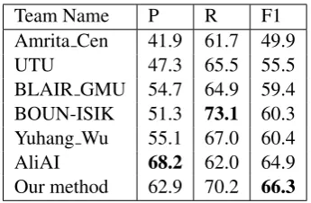
Table 3: The official results of the BB-rel task.

performances of our model were evaluated by the standard evaluation measures: precision (P), recall (R) and F1-score (F1).

3.2 Hyper-parameter

The hyper-parameter setting is listed in Table 2. We tuned hyper-parameters based on the develop-ment set.

3.3 Official Results

The official results on the test set are shown in Ta-ble 3. There are totally 7 teams participating in the BB-rel task. Each team could submit up to 2 predictions. We report the top results for all teams. As we can see, our method achieved the highest F1 (66.3%), and the second highest precision (62.9%) and recall (70.2%).

Figure 5: Ensemble training and inference.

3.4 Ensemble Training and Inference

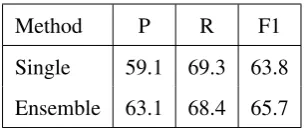
In relation extraction tasks, the ensemble training and inference have proven to be an effective way to improve performance of the neural network model (Mehryary et al.,2016;Lim and Kang,2018). Fol-lowing previous work (Lim and Kang,2018), we improve performance of our model using the en-semble training and inference. We sum the out-put probabilities (logits) of ensemble members, which are generated using the same neural net-work model but different weight initialization.

As shown in Figure5, M1 to M10 are the mod-els using the same structure and hyper-parameters. In the training phase, we independently trained each ensemble member with different initialized parameters. When inferring a relation for an easy sample, the trained ensemble members make rel-atively consistent predictions. When inferring for a difficult sample, the trained ensemble members may make different predictions. We incorporate the voting results of 10 ensemble members to pro-duce final results.

Method P R F1

Single 59.1 69.3 63.8

Ensemble 63.1 68.4 65.7

Table 4: Effects of ensemble training and inference.

Relation P R F1

Intra

Live in 61.6 60.0 60.8

Exhibits 73.4 80.6 76.8

Total 64.8 65.2 65.0

Intra+Inter

Live in 59.5 63.7 61.5

Exhibits 72.8 82.4 77.3

Total 63.1 68.4 65.7

Table 5: Results of recognizing inter- and intra-sentence relations.

3.5 Results of Recognizing Inter- and Intra-Sentence Relations

In this section, we discuss the performance of our model in Intra- and inter-sentence relation. As shown in Table 5, we obtained an F1-score of 65.0 when we only evaluated the intra-sentence re-lationships. When we evaluated both intra- and inter-sentence relationship, F1-score, Recall in-crease by 0.7% and 3.2% respectively. But Pre-cision drops by 1.7%. We can also see from the table that the performance of ”Exhibits” relation is better than the performance of the ”Live in” rela-tion. Because most of the ”Exhibits” relation hap-pen within a sentence and have a certain pattern.

3.6 Effects of Lexical Chains

In order to verify the effectiveness of construct-ing inter-sentence dependency graphs by lexical chains, we also conducted related experiments on development set. The experimental results are shown in Table 6. “lexical chains” denotes the model employing the proposed method that con-structs inter-sentence dependency graphs by lexi-cal chains. “root nodes” denotes the model where the inter-sentence dependency graphs are built us-ing root nodes. Table 6 shows the performance comparison of the “lexical chains” method and the “root nodes” method on the development set. The “lexical chains” method obtained better

perfor-Method P R F1

Root nodes 62.7 67.3 64.9

Lexical chains 63.1 68.4 65.7

Table 6: Effects of lexical chains.

Figure 6: Examples of false positives. The Red and green words denote Microorganism and Habitat entities respectively.

mance than the “root nodes” model. This demon-strates our idea is effective. The relevant sen-tences are usually expressed using relevant words. These relevant words found by lexical chains can be used as the associations to connect the depen-dency graphs of different sentences. Therefore, we can build an effective representation for an inter-sentence entity pair.

3.7 Error Analysis

4 Related Work

In the natural language processing community, there are a number of related competitions and tasks (Wei et al., 2015; N´edellec et al., 2013;

Del´eger et al.,2016). Most prior work focused on extracting the relations within one sentence, and ignored the relations beyond one sentence.

In the NLP community, it has proven to be ef-fective to combine linguistic features with neural networks for relation extraction (Zhou et al.,2015;

Miwa and Bansal, 2016). Bunescu et al. (2005) demonstrated that the relationship of an entity pair can be captured along their shortest dependency path in the dependency graph because the words on the shortest dependency path concentrate the most relevant information and diminish redundant information. Following this observation, several studies (Xu et al.,2015;Liu et al.,2015) achieved outstanding performance by combining shortest dependency paths with various neural networks. As deep learning develops, some attention-based neural architectures (Zhou et al.,2016;Lin et al.,

2016) have been proposed for relation classifica-tion and show the state-of-the-art performance. But with a few exceptions, almost all related work only focused on intra-sentence relation extraction, without considering the inter-sentence relations.

Recent work has explored some approaches to consider inter-sentence relations, such as Graph LSTMs (Peng et al., 2017), self-attention (Verga et al., 2018), Graph CNNs (Sahu et al., 2019). However, none of these work investigated lexical chains for inter-sentence relation extraction. In the future, we will evaluate our approach on some large-scale datasets for intra- and inter-sentence relation extraction (Yao et al.,2019).

5 Conclusion

In this paper, we describe our approach used for participating the Bacteria Biotope task at BioNLP-OST 2019. Our approach achieved very com-petitive performance in the official evaluation. We found that the idea using lexical chains to build inter-sentence dependency graphs is effec-tive. Moreover, ensemble training and inference can improve the performance of our model. The attention-guided graph convolution neural net-work performs well in extracting Bacteria Biotope relations. However, our approach is not specific to Bacteria Biotope relation extraction, and it can be applied to other relation extraction tasks.

Acknowledgments

References

Jari Bj¨orne and Tapio Salakoski. 2013.TEES 2.1: Au-tomated annotation scheme learning in the bionlp 2013 shared task. In Proceedings of the BioNLP Shared Task 2013 Workshop, Sofia, Bulgaria, August 9, 2013, pages 16–25.

Robert Bossy, Louise Del´eger, Estelle Chaix, Mouhamadou Ba, and Claire Nedellec. 2019. Bacteria Biotope at BioNLP Open Shared Tasks 2019. In Proceedings of the BioNLP Open Shared Tasks 2019 Workshop.

Robert Bossy, Wiktoria Golik, Zorana Ratkovic, Philippe Bessi`eres, and Claire N´edellec. 2013.

Bionlp shared task 2013 - an overview of the bac-teria biotope task. In Proceedings of the BioNLP Shared Task 2013 Workshop, Sofia, Bulgaria, August 9, 2013, pages 161–169.

Razvan C Bunescu and Raymond J Mooney. 2005. A shortest path dependency kernel for relation extrac-tion. InEMNLP, pages 724–731.

Louise Del´eger, Robert Bossy, Estelle Chaix, Mouhamadou Ba, Arnaud Ferre, Philippe Bessieres, and Claire Nedellec. 2016. Overview of the bacteria biotope task at bionlp shared task 2016. In Proceed-ings of the 4th BioNLP shared task workshop, pages 12–22.

Louise Del´eger, Robert Bossy, Estelle Chaix, Mouhamadou Ba, Arnaud Ferr´e, Philippe Bessi`eres, and Claire N´edellec. 2017. Overview of the bacteria biotope task at bionlp shared task 2016. In Bionlp Shared Task Workshop-association for Computational Linguistics.

Zhijiang Guo, Yan Zhang, and Wei. Lu. 2019a. Atten-tion guided graph convoluAtten-tional networks for rela-tion extracrela-tion. InACL.

Zhijiang Guo, Yan Zhang, Zhiyang Teng, and Wei Lu. 2019b. Densely connected graph convolutional networks for graph-to-sequence learning. TACL, 7:297–312.

Graeme Hirst and David St-Onge. 1997. Lexical chains as representations of context for the detection and correction of malapropisms. Lecture Notes in Physics, 728(9):123–149.

Sepp Hochreiter. 1998. The vanishing gradient lem during learning recurrent neural nets and prob-lem solutions. International Journal of Uncertainty, Fuzziness and Knowledge-Based Systems, 06(02):–.

Gao Huang, Zhuang Liu, Laurens van der Maaten, and Kilian Q. Weinberger. 2017. Densely connected convolutional networks. In CVPR, pages 2261– 2269.

J D Kim, S. Pyysalo, T. Ohta, R. Bossy, N. Nguyen, and J. Tsujii. 2011. Overview of bionlp shared task 2011. InBionlp Shared Task Workshop.

Jin Dong Kim, Tomoko Ohta, Sampo Pyysalo, Yoshi-nobu Kano, and Jun’Ichi Tsujii. 2009. Overview of bionlp’09 shared task on event extraction. In Work-shop on Current Trends in Biomedical Natural Lan-guage Processing: Shared Task.

Kenton Lee, Luheng He, Mike Lewis, and Luke Zettle-moyer. 2017. End-to-end neural coreference resolu-tion. InEMNLP, pages 188–197.

Jake Lever and Steven J. Jones. 2016. VERSE: event and relation extraction in the bionlp 2016 shared task. InProceedings of the 4th BioNLP Shared Task Workshop, BioNLP 2016, Berlin, Germany, August 13, 2016, pages 42–49.

Liunian Li, Xiaojun Wan, Jin-ge Yao, and Siming Yan. 2017. Leveraging diverse lexical chains to construct essays for chinese college entrance examination. In

IJCNLP.

Sangrak Lim and Jaewoo Kang. 2018. Chemical-gene relation extraction using recursive neural network.

Database, 2018:bay060.

Yankai Lin, Shiqi Shen, Zhiyuan Liu, Huanbo Luan, and Maosong Sun. 2016. Neural relation extrac-tion with selective attenextrac-tion over instances. InACL, pages 2124–2133.

Yang Liu, Furu Wei, Sujian Li, Heng Ji, Ming Zhou, and WANG Houfeng. 2015. A dependency-based neural network for relation classification. In ACL, pages 285–290.

Christopher D. Manning, Mihai Surdeanu, John Bauer, Jenny Finkel, Steven J. Bethard, and David Mc-closky. 2014. The stanford corenlp natural language processing toolkit. InMeeting of the Association for Computational Linguistics: System Demonstrations.

Laura Mascarell. 2017. Lexical chains meet word embeddings in document-level statistical machine translation. In Discourse in Machine Translation (DiscoMT).

Farrokh Mehryary, Jari Bj¨orne, Sampo Pyysalo, Tapio Salakoski, and Filip Ginter. 2016. Deep learning with minimal training data: Turkunlp entry in the bionlp shared task 2016. In Proceedings of the 4th BioNLP Shared Task Workshop, BioNLP 2016, Berlin, Germany, August 13, 2016, pages 73–81.

Makoto Miwa and Mohit Bansal. 2016. End-to-end re-lation extraction using lstms on sequences and tree structures. InACL, pages 1105–1116.

Jane Morris and Graeme Hirst. 1991. Lexical cohe-sion computed by thesaural relations as an indicator of the structure of text. Computational Linguistics, 17(1):21–48.

Claire N´edellec, Robert Bossy, Jin Dong Kim, Jung Jae Kim, Tomoko Ohta, Sampo Pyysalo, and Pierre Zweigenbaum. 2013. Overview of bionlp shared task 2013. InBionlp Shared Task Workshop.

Nanyun Peng, Hoifung Poon, Chris Quirk, Kristina Toutanova, and Wen-tau Yih. 2017. Cross-sentence n-ary relation extraction with graph LSTMs. Trans-actions of the Association for Computational Lin-guistics, 5:101–115.

S. Pyysalo, F. Ginter, H. Moen, T. Salakoski, and S. Ananiadou. 2013. Distributional semantics re-sources for biomedical text processing. In Proceed-ings of LBM 2013, pages 39–44.

Zorana Ratkovic, Wiktoria Golik, Pierre Warnier, Philippe Veber, and Claire N´edellec. 2011. Bionlp 2011 task bacteria biotope - the alvis system. In Pro-ceedings of BioNLP Shared Task 2011 Workshop, Portland, Oregon, USA, June 24, 2011, pages 102– 111.

Steffen Remus and Chris Biemann. 2013. Three knowledge-free methods for automatic lexical chain extraction. InNAACL.

Sunil Kumar Sahu, Fenia Christopoulou, Makoto Miwa, and Sophia Ananiadou. 2019. Inter-sentence relation extraction with document-level graph con-volutional neural network. In Proceedings of the 57th Annual Meeting of the Association for Com-putational Linguistics, pages 4309–4316, Florence, Italy. Association for Computational Linguistics.

Adam Santoro, David Raposo, David G. T. Barrett, Mateusz Malinowski, Razvan Pascanu, Peter W. Battaglia, and Tim Lillicrap. 2017. A simple neural network module for relational reasoning. InNIPS, pages 4967–4976.

Nicola Stokes, Joe Carthy, and Alan F. Smeaton. 2004. Select: a lexical cohesion based news story segmen-tation system. Ai Communications, 17(17):3–12.

Qian Tao, Donghong Ji, and Congling Xia. 2014. Word sense induction using lexical chain based hyper-graph model. InColing.

Ashish Vaswani, Noam Shazeer, Niki Parmar, Jakob Uszkoreit, Llion Jones, Aidan N. Gomez, Lukasz Kaiser, and Illia Polosukhin. 2017. Attention is all you need. InNIPS, pages 5998–6008.

Patrick Verga, Emma Strubell, and Andrew McCallum. 2018. Simultaneously self-attending to all mentions for full-abstract biological relation extraction. In

Proceedings of the 2018 Conference of the North American Chapter of the Association for Computa-tional Linguistics: Human Language Technologies, Volume 1 (Long Papers), pages 872–884.

Chih-Hsuan Wei, Yifan Peng, Robert Leaman, Al-lan Peter Davis, Carolyn J Mattingly, Jiao Li, Thomas C Wiegers, and Zhiyong Lu. 2015.

Overview of the biocreative v chemical disease re-lation (cdr) task. InProceedings of the fifth BioCre-ative challenge evaluation workshop, volume 14.

Yan Xu, Lili Mou, Ge Li, Yunchuan Chen, Hao Peng, and Zhi Jin. 2015. Classifying relations via long short term memory networks along shortest depen-dency paths. InEMNLP, pages 1785–1794.

Yuan Yao, Deming Ye, Peng Li, Xu Han, Yankai Lin, Zhenghao Liu, Zhiyuan Liu, Lixin Huang, Jie Zhou, and Maosong Sun. 2019. DocRED: A large-scale document-level relation extraction dataset. In Pro-ceedings of the 57th Annual Meeting of the Associa-tion for ComputaAssocia-tional Linguistics, pages 764–777, Florence, Italy. Association for Computational Lin-guistics.

Yuhao Zhang, Peng Qi, and Christopher D. Manning. 2018. Graph convolution over pruned dependency trees improves relation extraction. InEMNLP.

Hao Zhou, Yue Zhang, Shujian Huang, and Jiajun Chen. 2015. A neural probabilistic structured-prediction model for transition-based dependency parsing. InACL, pages 1213–1222.