Performance Optimization of Markov Models in Simulating Computer Networks

(1)

Performance Optimization of Markov Models in

Simulating Computer Networks

Abstract--This paper concerns the application of Discrete Markov models [1], [2] for the simulation of computer networks where the number of clients remains unchanged. Two numerical methods [3] has been used, the Power simulation method and the P-simulation method. Two network models has been used the Gordan-Newell and the Cox-Cox models. In simulating those two models, the asymptotic performance of the simulation has been compared, in term of the convergence criteria toward the stationary state of the model.

Index Terms— Computer Networks Simulation, Discrete Markov Chains, Performance evaluation, P-simulation, Power simulation.

I. INTRODUCTION

Computer networks belong to a class of physical systems that can be studied effectively by means of discrete events simulation models. The computer network subject of the simulation is the closed network “Gordan-Newell network” and “Cox-Cox network” with a constant number of clients.

Considering the fact that the state of the network is described in terms of numerical behavior values, computer network falls in the category of memory less behavior because the knowledge of the present decouples the past from the future. Though exploring the behavior of computer networks through Markov models is legal, because Markov chain is a special stochastic process in which the future probabilistic behavior of the process is uniquely determined by its present state.

Network entities such as the access behaviors to the network may be described in the form of discrete chain events. Two types of Markov chain models will be applied in the simulation, the Power Markov process and the P-simulation Markov process in a discrete state space.

The two method’s convergence to the stationary state will be compared in order to find which method is more reliable for the simulation of the Gordan-Newell and Cox-Cox network models.

F. Nisrine Sinno is in the Computer and Applied Mathemetics Department, At the faculty of Sciences, Lebanese University, e-mail: [email protected]. S. Hussein Youssef is in the department of Physique des materiaux , Faculty of Sciences, Lebanese University.

T.Ghaddar Ahmad is in the Computer and Applied Mathemetics Department,

At the faculty of Sciences, Lebanese University

II. SIMULATION MODELS

A. Discrete Time Markov Model

A discrete time Markov model is defined in terms of a set of transition probabilities between the discrete states of the model. Transitions are associated with transition probabilities between states.

The NxN transition probabilities between N states is called the Transition Probability Matrix P.

If P0 is the initial probability vector then the state probability after k steps is given by the vector :

π

_k=P0* k

P

(1)

the matrix k

P

is the k -th transition matrix after multiplying P to itself , k times.

At steady state no more changes in states probabilities are expected when P is multiplied by the current probability P vector, this is because the Markov chain is ergodic [3]. The steady state probability vector in all states of the Markov Model is such that:

Π x P= Π (2) This equation will be used along with the condition

∑

n₌

i 0

π

i = 1 (3)

in order to determine all the steady state probabilities for the chosen network models.

B. Gordan-Newell Network [4]

It is a network designed with a constant number of clients. The number of possible states is limited. The network is composed of several nodes. Supposing that m is the number of nodes, and n is the constant number of packets traveling in the network sent by n different clients, N possible states is given by :

N=

_C

m n m

1 1

− +

− (4)

The set of possible states for a three nodes network is given by:

(2)

2 )

2 )(

1 (

2 2

+

=

+

n

C

E

N

n (6)

The Gordan-Newell network model is illustrated in the Fig. 1 below.

The number of states of the network increase rapidly with n. If the number of packets accessing the nodes of the network is n=2, the number of states will be 6 distributed among the three nodes, the states are:

(2,0,0),(1,1,0),(0,2,0) ,(1,0,1),(0,0,2),(0,1,1).

With the stochastic variable a such as (0<a<1), during the time [t,t+1] the Bernouilli variable with parameter a is the number of packets accessing the network.

Defining A(t)=1 as the number of packets accessing the node during [t,t+1], and A(t)=0 as number of packets not accessing the node during that interval,

the probability to have A(t) packets accessing one node will be:

P[A(t) =1] = a (7) and the probability not to have A(t) packets accessing one

node is:

P[A(t)=0] = 1-a. (8) In Fig.1 in three nodes network, i will be the number of

packets accessing node 1, with the probability μ ₁ , j will be the number of packets accessing node 2 with the probability

μ

₂, k will be the number of packets accessing node 3 with the probability

μ

₃,

The total number n of packets accessing the network is constant with n=i+ j+ k. The packets in node 1 can either access node 2 with probability a or access node 3 with probability 1-a, packets in node 2 can access node 1 with probability 1, packets in node 3 can access node 1 with probability 1.

The states diagram for Gordan-Newell network, with 2 packets (clients) is given Fig.2.

Figure 2. States diagram for Gordan-Newell network with 2 clients

In order to construct an algorithm to memorize the state of node I at a certain time t ,we consider that i

t

X

is the number of clients at that moment in node I, the vector

)

,

(

1 2 3

t t t

t

X

G

=

will represent the set of clients

present at nodes 1,2,3 at time t in the network .

First theorem:

X

_t

G

is finite, homogeneous, irreducible [1]

Second theorem: the steady state probability vector for any

state I (i,j,k) is given by:

k

j

i

k

j

i

G

1

2

3 ,

,

1 _ζ

_ζ

π

=

(9)

with

∑

π

_i_,_j_,_k= 1 (10) If Di defines the average rate of clients accessing node i,

at steady state then :

D1 = D2 + D3, D2 = a.D1, D3 = (1-a).D1 (11)

This system is linear, homogeneous and irreducible, it has at least one solution. One solution is: ( x, ax, (1-a)x ).

The steady state probability for an average rate of clients x in node 1, a*x in node 2, (1-a)*x in node 3 is respectively :

∑

= + +

=

n k j i k j i

G

x

.

/

1 ,

/

3 2 1 3 3 2 2 1 1

ζ

μ

ζ

μ

ζ

μ

ζ

(12)

Considering the matrix Q[N,N] of the steady state probabilities , with N=6 states according to the 2 clients Gordan-Newell network Fig.2 , Q will have the dimensions [6,5] . In every row of the matrix, one column element is null .

if every state I is defined by i and j then k is deduced from

µ2

1

2 µ1

µ3

a

1-a

j

k

(3)

i , j , n

k=n-(i+j). (13) In order to simulate the network according to the Power

and P-simulation methods, algorithms converting from state I into the form (i,j) and from the form (i,j) into state I has been constructed (extracting line, then column, then line with restriction, then column with restriction ..). We will increment I from 0 to N-1 by incrementing i from 0 to N and incrementing j from 0 to N-i.

C. The Cox-Cox network model[5]

In this model the network has constant number of clients, but the transition probability matrix P varies according to a certain coefficient given by construction.

[image:3.595.320.552.376.634.2]

The model is represented in the following Fig.3, it is the “Coaxian” server representing two computer networks A, B with respectively coefficient λ and the number of nodes m for A, and for B coefficient µ with number of nodes n. The simulation of this model will show the convergence performance in extreme cases of an organized transition probability matrix and a disturbed one by modifying the coefficients.

Figure 3. States Diagram for Coaxian server (with 2 networks A,B)

Theorems:

Steady state probability matrix in A is :

π

_A

=

π

₁

+

π

₂

+..+

π

m

(14) Steady state probability matrix in B is :

π

_B

=

π

m

+

1

+

π

m

+

2

+..+

π

m

+

n

(15)

A

π

= µ / (λ+µ) and

π

_B

= λ/ (λ+µ)

∀

k

(16)

III. TESTS AND RESULTS

A. Gordan-Newell Network simulation

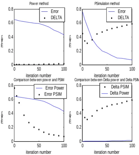
Tests have been made using over 10000 stochastic data entries. Fig.[4] [5] [6] [7] show that the method P-simulation is more efficient than the Power simulation method because the convergence to the stationary state is quicker

with P-simulation.

0 50 100

0 0.2 0.4 0.6 0.8

iteration number Err

or

Pow er method

0 50 100

0 0.2 0.4 0.6 0.8

or

PSimulation method

0 50 100

0 0.2 0.4 0.6 0.8

or

Comparison betw een pow er and PSIM

0 50 100

0 0.2 0.4 0.6 0.8

or

Comparison betw een Delta pow er and Delta PSIM

Delta PSIM Delta Power Error Power

Error PSIM

Error DELTA Error

DELTA

Figures [4][5][6][7] Comparison between Power and

P-simulation of the Gordan-Newell Network with

2 clients.

B. Cox-Cox Model simulation

Several models of Cox-Cox networks has been simulated by changing the coefficients. Three models simulations

A

m

λ

λ λ λ

λ .

2

k

λ .

1

k ki.λ

μμ μ

.

1

k′ _._μ

2

(4)

[image:4.595.311.553.83.304.2]

are shown in the figures 8,9,10: The normal network model Fig.9, the organized model (Fig.10) and the disturbed model (Fig.8).

The steady state probability matrixes

π

_A

and

π

_B

are calculated using the Markov chain P-simulation and Power simulation methods [6, 7].

Figure 8. Error in a Disturbed Model Simulation

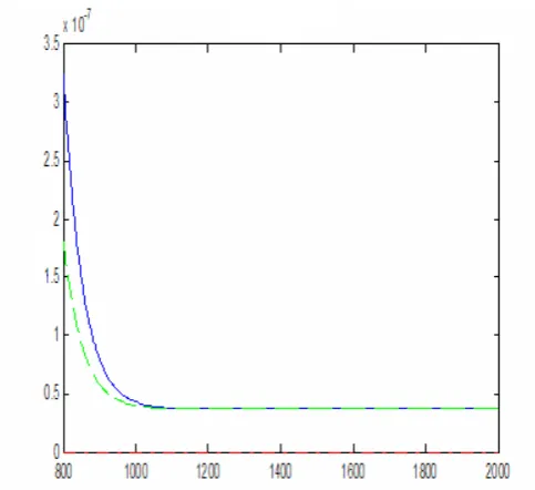
Figure 9. Error in normal Cox-Cox Model with

normalized power simulation method

Figure 10. Error in an Organized Model Simulation

[image:4.595.66.281.177.395.2]

The first Fig .8 shows the disturbed model , the second Fig.9

shows the case of a normal network, while the third Fig.10 represents the results for the organized model. The first conclusion is that the coefficients play a major role:

Case of the disturbed Cox-Cox model Fig. 8 : The Power method seems to converge rapidly at the beginning of the iterations, but the P-simulation method leads to a more accurate simulation, the error at the end of the iterations is less than the one in the Power simulation method.

Case of an organized Cox-Cox model Fig.10: In this model, the Power method converges rapidly to the stable state comparing to the P-simulation method. But comparing to the results with the disturbed model (Fig.8), the –simulation convergence is much slower.

Case of a normal Cox-Cox model with normalized power simulation and p-simulation Fig.9 : Same conclusion as for the disturbed model, but with the normalized power simulation method the convergence is more accurate than with the P-simulation method..

Those results let us conclude that:

• Organized models simulation is less convergent than disturbed and normal models.

• That the normalized power simulation method is more accurate than the power simulation method without normalization.

(5)

In order to confirm this conclusion, the tests of the simulations

where done using Matlab and C++ for up to 100 iterations in case of a normal Cox-Cox model. We found the following results:

• Errpsim (matlab) < Errpower (Matlab) without normalization

• Errpsim (C++_{) < Errpower (C}++_{) without}

normalization

• Errpower (C++_{) with normalization < Errpower}

(Matlab) with normalization

So for certain models the error in normalized Power simulation method is less than the one obtained when using the P-simulation method but this assumption cannot be generalized.

V. CONCLUSION

The paper has described the comparison of the asymptotic performance between the P-simulation method and the Power simulation method for several cases of networks, the Gordan-Newell network and different kinds of Cox-Cox models. The analysis of the results leads to the following conclusions:

• The convergence acceleration of P-simulation depends on the state extracted from the set E of chosen states.

• P-simulation converges toward accurate solutions better than with the Power simulation method.

• Normalization of the Power simulation method in case of disturbed Cox-Cox models is more efficient than the P-simulation method.

Increasing the asymptotic performance in Markov chains of high dimension is an open access problem. The simulation methods proposed in this paper help in understanding the behavior according to several Markov chains simulation of computer networks. But more tests on other kind of networks are needed in order to evaluate the simulation methods used.

REFERENCES

[1] Bloch, Grenier, Hermann and Trivedi, « Queuing Network and Markov Chain », J. Wiley ed. 1998.

[2] A.Bouillard. « Optimisation et analyse probabiliste de systèmes à événements discrets ». PhD thesis, ENS Lyon, France, 2005.

[3] P.Fernandes.« Méthodes numériques pour la solution de systèmes Markoviens à grand espace d'états ». PhD thesis, INPG, Grenoble, France, 1998.

[4] Kishor, Shridharbhai and Trivedi, « Probability & statistics with reliability queuing and computer science applications », PRENTICE-HALL, INC., Englewood Cliffs, New Jersey 07632.

[5] William J. Stewart. « Introduction to the numerical solution of Markov Chains». Princeton University Press, new Jersey 1994.

[6] Pellaumail, Boyer, Leguesdron « Réseaux ATM et P-simulation». [7] A.Bouillard. « Optimisation et analyse probabiliste de systèmes à

événements discrets ». PhD thesis, ENS Lyon, France, 2005.