Large Scale Stochastic Sampling from the Probability Simplex

Large-Scale Stochastic Sampling from the Probability

Simplex

Jack Baker

STOR-i CDT, Deptment of Mathematics and Statistics Lancaster University

[email protected]

Paul Fearnhead

Department of Mathematics and Statistics Lancaster University

Emily B. Fox Department of Statistics University of Washington

Christopher Nemeth

Department of Mathematics and Statistics Lancaster University

Abstract

Stochastic gradient Markov chain Monte Carlo (SGMCMC) has become a popular method for scalable Bayesian inference. These methods are based on sampling a discrete-time approximation to a continuous time process, such as the Langevin diffusion. When applied to distributions defined on a constrained space, such as the simplex, the time-discretisation error can dominate when we are near the boundary of the space. We demonstrate that while current SGMCMC methods for the simplex perform well in certain cases, they struggle withsparse simplex spaces; when many of the components are close to zero. However, most popular large-scale applications of Bayesian inference on simplex spaces, such as network or topic models, are sparse. We argue that this poor performance is due to the biases of SGMCMC caused by the discretization error. To get around this, we propose the stochastic CIR process, which removes all discretization error and we prove that samples from the stochastic CIR process are asymptotically unbiased. Use of the stochastic CIR process within a SGMCMC algorithm is shown to give substantially better performance for a topic model and a Dirichlet process mixture model than existing SGMCMC approaches.

1

Introduction

Stochastic gradient Markov chain Monte Carlo (SGMCMC) has become a popular method for scalable Bayesian inference (Welling and Teh, 2011; Chen et al., 2014; Ding et al., 2014; Ma et al., 2015). The foundation of SGMCMC methods are a class of continuous processes that explore a target distribution—e.g., the posterior—using gradient information; these processes converge to a Markov chain which samples from the posterior distribution exactly. SGMCMC methods replace the costly full-data gradients with minibatch-based stochastic gradients, which provides one source of error. Another source of error arises from the fact that the continuous processes are almost never tractable to simulate; instead, discretizations are relied upon. In the non-SG scenario, the discretization errors are corrected for using Metropolis-Hastings corrections. However, this is not (generically) feasible in the SG setting. The result of these two sources of error is that SGMCMC targets an approximate posterior (Welling and Teh, 2011; Teh et al., 2016; Vollmer et al., 2016).

Another significant limitation of SGMCMC methods is that they struggle to sample from constrained spaces. Naively applying SGMCMC can lead to invalid, or inaccurate values being proposed. The result is large errors near the boundary of the space (Patterson and Teh, 2013; Ma et al., 2015; Wenzhe Li, 2016). A particularly important constrained space is the simplex space, which is used to model discrete probability distributions. A parameterωof dimensiondlies in the simplex if it satisfies the following conditions: ωj ≥0for allj = 1, . . . , dandP

d

j=1ωj = 1. Many popular

models contain simplex parameters. For example, latent Dirichlet allocation (LDA) is defined by a set of topic-specific distributions on words and document-specific distributions on topics. Probabilistic network models often define a link probability between nodes. More generally, mixture and mixed membership models have simplex-constrained mixture weights; even the hidden Markov model can be cast in this framework with simplex-constrained transition distributions. As models become large-scale, these vectorsωoften becomesparse–i.e., manyωjare close to zero—pushing them to

the boundaries of the simplex. All the models mentioned have this tendency. For example in network data, nodes often have relatively few links compared to the size of the network, e.g., the number of friends the average social network user has will be small compared with the size of the whole social network. In these cases the problem of sampling from the simplex space becomes evenharder; since many values will be very close to the boundary of the space.

Patterson and Teh (2013) develop an improved SGMCMC method for sampling from the probability simplex: stochastic gradient Riemannian Langevin dynamics (SGRLD). The improvements achieved are through an astute transformation of the simplex parameters, as well as developing a Riemannian (see Girolami and Calderhead, 2011) variant of SGMCMC. This method achieved state-of-the-art results on an LDA model. However, we show despite the improvements over standard SGMCMC, the discretization error of this method still causes problems on the simplex. In particular, it leads to asymptotic biases which dominate at the boundary of the space and causes significant inaccuracy. To counteract this, we design an SGMCMC method based on the Cox-Ingersoll-Ross (CIR) process. The resulting process, which we refer to as the stochastic Cox-Ingersoll-Ross process (SCIR), hasno discretization error. This process can be used to simulate from gamma random variables directly, which can then be moved into the simplex space using a well known, standard transformation. The CIR process has a lot of nice properties. One is that the transition equation is known exactly, which is what allows us to simulate from the process without discretization error. We are also able to characterize important theoretical properties of the SCIR algorithm, such as the non-asymptotic moment generating function, and thus its mean and variance.

We demonstrate the impact of this SCIR method on a broad class of models. Included in these experiments is the development of a scalable sampler for Dirichlet processes, based on the slice sampler of Walker (2007); Papaspiliopoulos (2008); Kalli et al. (2011). To our knowledge the application of SGMCMC methods to Bayesian nonparametric models has not been explored, and we consider this a further contribution of the article. All proofs in this article are relegated to the Supplementary Material. All code for the experiments will be made available online, and full details of hyperparameter and tuning constant choices has been detailed in the Supplementary Material.

2

Stochastic Gradient MCMC on the Probability Simplex

2.1 Stochastic Gradient MCMC

Consider Bayesian inference for continuous parametersθ∈_Rd_{based on datax={x}

i}Ni=1. Denote

the density ofxiasp(xi|θ)and assign a prior onθwith densityp(θ). The posterior is then defined,

up to a constant of proportionality, asp(θ|x)∝p(θ)QN

i=1p(xi|θ), and has distributionπ. We define

f(θ) :=−logp(θ|x). Whilst MCMC can be used to sample fromπ, such algorithms require access to the full data set at each iteration. Stochastic gradient MCMC (SGMCMC) is an approximate MCMC algorithm that reduces this per-iteration computational and memory cost by using only a small subset of data points at each step.

The most common SGMCMC algorithm is stochastic gradient Langevin dynamics (SGLD), first introduced by Welling and Teh (2011). This sampler uses the Langevin diffusion, defined as the solution to the stochastic differential equation

dθt=−∇f(θt)dt+

√

whereWtis ad-dimensional Wiener process. Similar to MCMC, the Langevin diffusion defines a

Markov chain whose stationary distribution isπ.

Unfortunately, simulating from (2.1) is rarely possible, and the cost of calculating∇fisO(N)since it involves a sum over all data points. The idea of SGLD is to introduce two approximations to circumvent these issues. First, the continuous dynamics are approximated by discretizing them, in a similar way to Euler’s method for ODEs. This approximation is known as theEuler-Maruyama method. Next, in order to reduce the cost of calculating∇f, it is replaced with a cheap, unbiased estimate. This leads to the following update equation, with user chosen stepsizeh

θm+1=θm−h∇fˆ(θ) +

√

2hηm, ηm∼N(0,1). (2.2)

Here,∇fˆis an unbiased estimate of∇fwhose computational cost isO(n)wherenN. Typically, we set∇fˆ(θ) :=−∇logp(θ)−N/nP

i∈Sm∇logp(xi|θ), whereSm⊂ {1, . . . , N}resampled at each iteration with|Sm|=n. Applying (2.2) repeatedly defines a Markov chain that approximately

targetsπ(Welling and Teh, 2011). There are a number of alternative SGMCMC algorithms to SGLD (Chen et al., 2014; Ding et al., 2014; Ma et al., 2015), based on approximations to other diffusions that also target the posterior distribution.

Recent work has investigated reducing the error introduced by approximating the gradient using minibatches (Dubey et al., 2016; Nagapetyan et al., 2017; Baker et al., 2017; Chatterji et al., 2018). While, by comparison, the discretization error is generally smaller, in this work we investigate an important situation where it degrades performance considerably.

2.2 SGMCMC on the Probability Simplex

We aim to make inference on the simplex parameter ω of dimension d, where ωj ≥ 0 for all

j = 1, . . . , dand Pd

j=1ωj = 1. We assume we have categorical datazi of dimension dfor

i = 1, . . . , N, sozij will be 1 if data pointibelongs to categoryj andzikwill be zero for all

k 6= j. We assume a Dirichlet prior Dir(α)onω, with densityp(ω) ∝ Qd

j=1ω

αj

d , and that the

data is drawn fromzi|ω∼Categorical(ω)leading to a Dir(α+PN_i=1zi)posterior. An important

transformation we will use repeatedly throughout this article, is that if we havedrandom gamma variablesXj ∼Gamma(αj,1). Then(X1, . . . , Xd)/PjXjwill have Dir(α)distribution, where

α= (α1, . . . , αd).

In this simple case the posterior ofωcan be exactly calculated. However, in the applications we consider theziare latent variables, and they are also simulated as part of a larger Gibbs sampler. Thus

theziwill change at each iteration of our algorithm. We are interested in the situation where this is

the case, andNis large, so that standard MCMC runs prohibitively slowly. The idea of SGMCMC in this situation is to use sub-samples of thezis to propose appropriate local-moves toω.

Applying SGMCMC to models which contain simplex parameters is challenging due to their con-straints. Naively applying SGMCMC can lead to invalid values being proposed. The first work to introduce an SGMCMC algorithm specifically for the probability simplex was Patterson and Teh (2013), the algorithm is a variant of SGLD known as stochastic gradient Riemannian Langevin dynamics (SGRLD). Patterson and Teh (2013) try a variety of transformations forωwhich will move the problem onto a space inRd, where standard SGMCMC can be applied. They also build

upon standard SGLD by developing a Riemannian variant (see Girolami and Calderhead, 2011). Riemannian MCMC takes into account the geometry of the space, which assisted with errors at the boundary of the space. The parameterisation Patterson and Teh (2013) find numerically performs the best is ωj = |θj|/Pd_j=1|θj|. They use a mirrored gamma prior forθj, which has density

p(θj)∝ |θj|αj−1e−|θj|. This means the prior forωremains the required Dirichlet distribution. They

calculate the density ofzigivenθusing a change of variables and use an SGLD update to calculateθ.

2.3 SGRLD on Sparse Simplex Spaces

Patterson and Teh (2013) suggested that the boundary of the space is where most problems occur using these kind of samplers. In many popular applications, such as LDA and modeling sparse networks, some of the componentsωjwill be close to 0, referred to as asparsespace. In other words,

there will be manyjfor whichPN

● ● ● ● ● ● ● ● ● ● ● ● ● ● ● ● ● ● ● ● ● ● ● ● ● ● ● ● ● ● ● ● ● ● ● ● ● ● ● ● ● ● ● ● ● ● ● ● ● ● ● ● ● ● ● ● ● ● ● ● ● ● ● ● ● ● ● ● ● ● ● ● ● ● ● ● ● ● ● ● ● ● ● ● ● ● ● ● ● ● ● ● ● ● ● ● ● ● ● ● ● ● ● ● ● ● ● ● ● ● ● ● ● ● ● ● ● ● ● ● ● ● ● ● ● ● ● ● ● ● 1e−26 1e−19 1e−12 1e−05

Exact SCIR SGRLD

Method Omega Method Exact SCIR SGRLD

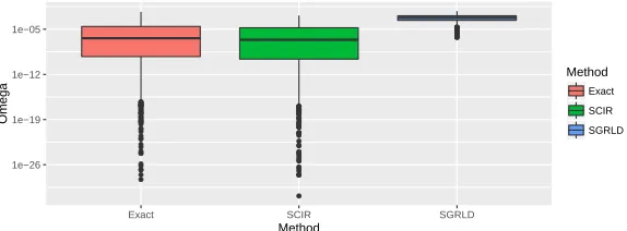
Figure 1: Boxplots of a 1000 iteration sample from SGRLD and SCIR fit to a sparse Dirichlet posterior, compared to 1000 exact independent samples. On the log scale.

Riemannian ideas to their SGLD algorithm. In order to demonstrate the problems with using SGRLD in this case, we provide a similar experiment to Patterson and Teh (2013). We use SGRLD to simulate from a sparse simplex parameterωof dimension ten with N = 1000. We setPN

i=1zi1 = 800,

PN

i=1zi2=P

N

i=1zi3= 100, andP

N

i=1zij = 0, for3< j≤10. The prior parameterαwas set to

0.1for all components. Leading to a highly sparse Dirichlet posterior. We will refer back to this experiment as therunning experiment. In Figure 1 we provide boxplots from a sample of the fifth component ofωusing SGRLD after 1000 iterations with 1000 iterations of burn-in, compared with boxplots from an exact sample. The method SCIR will be introduced later. We can see from Figure 1 that SGRLD rarely proposes small values ofω. This becomes a significant issue for sparse Dirichlet distributions, since the lack of small values leads to a poor approximation to the posterior; as we can see from the boxplots.

We hypothesize that the reason SGRLD struggles when ωj is near the boundary is due to the

discretization byh, and we now try to diagnose this issue in detail. The problem relates to the bias of SGLD, caused by the discretization of the algorithm. We use the results of Vollmer et al. (2016) to characterize this bias for a fixed stepsizeh. For similar results when the stepsize scheme is decreasing, we refer the reader to Teh et al. (2016). Proposition 2.1 is a simple application of Vollmer et al. (2016, Theorem 3.3), so we refer the reader to that article for full details of the assumptions. For simplicity of the statement, we assume thatθis 1-dimensional, but the results are easily adapted to thed-dimensional case.

Proposition 2.1. (Vollmer et al., 2016) Under Vollmer et al. (2016, Assumptions 3.1 and 3.2), assume

θ is 1-dimensional. Letθm be iterationmof an SGLD algorithm form = 1, . . . , M, then the

asymptotic bias defined bylimM→∞

1/M

PM

m=1E[θm]−Eπ[θ]

has leading termO(h).

While ordinarily this asymptotic bias will be hard to disentangle from other sources of error, asEπ[θ]

gets close to zero,hwill have to be set prohibitively small to give a good approximation toθ. The crux of the issue is that, while theabsolute errorremains the same, at the boundary of the space therelative erroris large sinceθis small, and biased upwards due to the positivity constraint. To counteract this, in the next section we introduce a method which has no discretization error. This allows us to prove that the asymptotic bias, as defined in Proposition 2.1, will be zero for any choice of stepsizeh.

3

The Stochastic Cox-Ingersoll-Ross Algorithm

We now wish to counteract the problems with SGRLD on sparse simplex spaces. First, we make the following observation: rather than applying a reparameterization of the prior forω; we can model the posterior forθjdirectly and independently asθj|z∼Gamma(αj+P

N

i=1zij,1). Then using the

gamma reparameterizationω=θ/P

jθjstill leads to the desired Dirichlet posterior. This leaves the

θjin a much simpler form, and this simpler form enables us to remove all discretization error. We do

processθtwith parameteraand stationary distribution Gamma(a,1)has the following form

dθt= (a−θt)dt+

p

2θtdWt. (3.1)

The standard CIR process has more parameters, but we found changing these made no difference to the properties of our proposed scalable sampler and so we omit them (for exact details see the Supplementary Material).

The CIR process has many nice properties. One that is particularly useful for us is that thetransition densityis known exactly. Defineχ2(ν, µ)to be the non-central chi-squared distribution with ν

degrees of freedom and non-centrality parameterµ. If at timetwe are at stateϑt, then the probability

distribution ofθt+his given by

θt+h|θt=ϑt∼

1−e−h

2 W, W ∼χ

2

2a,2ϑt

e−h

1−e−h

. (3.2)

This transition density allows us to simulate directly from the CIR process with no discretization error. Furthermore, it has been proved that the CIR process is negative with probability zero (Cox et al., 1985), meaning we will not need to take absolute values as is required for the SGRLD algorithm.

3.1 Adapting for Large Datasets

The next issue we need to address is how to sample from this process when the dataset is large. Suppose thatzi is data fori = 1, . . . , N, for some largeN, and that our target distribution is

Gamma(a,1), wherea=α+PN

i=1zi. We want to approximate the target by simulating from the

CIR process using only a subset ofzat each iteration. A natural thing to do would be at each iteration to replaceain the transition density equation (3.2) with an unbiased estimateˆa=α+N/nP

i∈Szi,

whereS⊂ {1, . . . , N}, similar to SGLD. We will refer to a CIR process using unbiased estimates in this way as the stochastic CIR process (SCIR). Fix some stepsizeh, which now determines how oftenˆais resampled rather than the granularity of the discretization. Supposeθˆmfollows the SCIR

process, then it will have the following update

ˆ

θm+1|θˆm=ϑm∼

1−e−h

2 W, W ∼χ

2

2ˆam,2ϑm

e−h

1−e−h

, (3.3)

whereˆam=α+N/nPi∈Smzi.

We can show that this algorithm will approximately target the true posterior distribution in the same sense as SGLD. To do this, we draw a connection between the SCIR process and an SGLD algorithm, which allows us to use the arguments of SGLD to show that the SCIR process will target the desired distribution. More formally, we have the following relationship:

Theorem 3.1. Letθtbe a CIR process with transition 3.2. ThenUt:=g(θt) = 2

√

θtfollows the

Langevin diffusion for a generalized gamma distribution.

Theorem 3.1, allows us to show that applying the transformationg(·)to the approximate SCIR process, leads to a discretization free SGLD algorithm for a generalized gamma distribution. Similarly, applyingg−1_{(·)to the approximate target of this SGLD algorithm leads to the desired Gamma(a,1)}

0.1 0.2 0.3 0.4

0.001 0.010 0.100

Minibatch Size (log scale)

KS Distance

(a)

0.1 0.2 0.3 0.4 0.5

0.001 0.010 0.100

Minibatch Size (log scale)

KS Distance

Method

Exact SCIR SGRLD

(b)

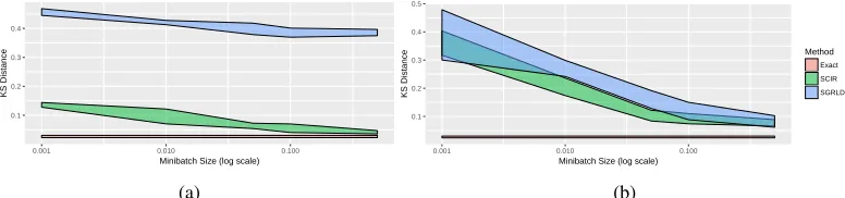
Figure 2: Kolmogorov-Smirnov distance for SGRLD and SCIR at different minibatch sizes when used to sample from (a), a sparse Dirichlet posterior and (b) a dense Dirichlet posterior.

Algorithm 1 below summarizes how SCIR can be used to sample from the simplex parameter

ω|z∼Dir(α+PN

i=1zi). This can be done in a similar way to SGRLD, with the same per-iteration

computational cost, so the improvements we demonstrate later are essentially for free.

Algorithm 1:Stochastic Cox-Ingersoll-Ross (SCIR) for sampling from the probability simplex. Input:Starting pointsθ0, stepsizeh, minibatch sizen.

Result:Approximate sample fromω|z. for m= 1toMdo

Sample minibatchSmfrom{1, . . . , N}

for j= 1toddo

Setˆaj←α+N/nPi∈Smzij.

Sampleθˆmj|θˆ(m−1)jusing (3.3) with parameterˆajand stepsizeh.

end

Setωm←θm/Pjθmj.

end

3.2 SCIR on Sparse Data

We test the SCIR process on two synthetic experiments. The first experiment is the running experiment on the sparse Dirichlet posterior of Section 2.3. The second experiment allocates 1000 datapoints equally to each component, leading to a highly dense Dirichlet posterior. For both experiments, we run 1000 iterations of optimally tuned SGRLD and SCIR algorithms and compare to an exact sample. For the sparse experiment, Figure 1 shows boxplots of samples from the fifth component ofω, which is sparse. For both experiments, Figure 2 plots the Kolmogorov-Smirnov distance (dKS) between

the approximate samples and the true posterior (full details of the distance measure are given in the Supplementary Material). For the boxplots, a minibatch of size 10 is used; for thedKSplots the

proportion of data in the minibatch is varied from 0.001 to 0.5. ThedKSplots show the runs of five

different seeds, which gives some idea of variability.

The boxplots of Figure 1 demonstrate that the SCIR process is able to handle smaller values ofω

much more readily than SGRLD. The impact of this is demonstrated in Figure 2a, the sparsedKS

plot. Here the SCIR process is achieving much better results than SGRLD, and converging towards the exact sample at larger minibatch sizes. The densedKSplot of Figure 2b shows that as we move

to the dense setting the samplers have similar properties. The conclusion is that the SCIR algorithm is a good choice of simplex sampler for either the dense or sparse case.

4

Theoretical Analysis

In the following theoretical analysis we wish to target a Gamma(a,1) distribution, wherea =

α+PN

i=1zifor some dataz. We run an SCIR algorithm with stepsizehforM iterations, yielding

the sampleθˆm for m = 1, . . . , M. We compare this to an exact CIR process with stationary

us to quantify the moments ofθˆmin the analysis to follow. For simplicity, we fix a stepsizehand,

abusing notation slightly, setθmto be a CIR process that has been run for timemh.

Theorem 4.1. LetθˆM be the SCIR process defined in(3.3)starting fromθ0afterM steps with

stepsizeh. LetθM be the corresponding exact CIR process, also starting fromθ0, run for timeM h,

and with coupled noise. Then the MGF ofθˆM is given by

MθˆM(s) =MθM(s)

M

Y

m=1

_1−s(1−e−mh₎

1−s(1−e−(m−1)h₎

−(ˆam−a)

, (4.1)

where we have

MθM(s) =

1−s(1−e−M h)−aexp

θ0

se−M h

1−s(1−e−M h₎

.

The proof of this result follows by induction from the properties of the non-central chi-squared distribution. The result shows that the MGF of the SCIR can be written as the MGF of the exact underlying CIR process, as well as an error term in the form of a product. Deriving the MGF enables us to find the non-asymptotic bias and variance of the SCIR process, which is more interpretable than the MGF itself. The results are stated formally in the following Corollary.

Corollary 4.2. Given the setup of Theorem 4.1,

E[ˆθM] =E[θM] =θ0e−M h+a(1−eM h),

so that, sinceEπ[θ] =a, thenlimM→∞|M1

PM

m=1E[ˆθm]−Eπ[θ]|= 0and SCIR is asymptotically

unbiased. Similarly,

Var[ˆθM] =Var[θM] + (1−e−2M h)

1−e−h

1 +e−hVar[ˆa],

whereVar[ˆa] =Var[ˆam]form= 1, . . . , Mand

Var[θM] = 2θ0(e−M h−e−2M h) +a(1−e−M h)2.

The results show that the approximate process is asymptotically unbiased. We believe this explains the improvements the method has over SGRLD in the experiments of Sections 3.2 and 5. We also obtain the non-asymptotic variance as a simple sum of the variance of the exact underlying CIR process, and a quantity involving the variance of the estimateˆa. This is of a similar form to the strong error of SGLD (Sato and Nakagawa, 2014), though without the contribution from the discretization. The variance of the SCIR is somewhat inflated over the variance of the CIR process. Reducing this variance would improve the properties of the SCIR process and would be an interesting avenue for further work. Control variate ideas could be applied for this purpose (Nagapetyan et al., 2017; Baker et al., 2017; Chatterji et al., 2018) and they may prove especially effective since the mode of a gamma distribution is known exactly.

5

Experiments

5.1 Latent Dirichlet Allocation

Latent Dirichlet allocation (LDA, see Blei et al., 2003) is a popular model used to summarize a collection of documents by clustering them based on underlying topics. The data for the model is a matrix of word frequencies, with a row for each document. LDA is based on a generative procedure. For each documentl, a discrete distribution over theKpotential topics,θl, is drawn asθl∼Dir(α)

for some suitably chosen hyperparameterα. Each topickis associated with a discrete distribution

φkover all the words in a corpus, meant to represent the common words associated with particular

topics. This is drawn asφk∼Dir(β), for some suitableβ. Finally, each word in documentlis drawn

a topickfromθland then the word itself is drawn fromφk.

LDA is a good example for this method becauseφkis likely to be very sparse, there are many words

1500 1600 1700 1800

0 10000 20000 30000 40000

Number of Documents

P

er

ple

xity

(a)

12.000 12.025 12.050 12.075 12.100

0 250 500 750 1000

Iteration

T

est Log Predictiv

e

Method SCIR SGRLD

(b)

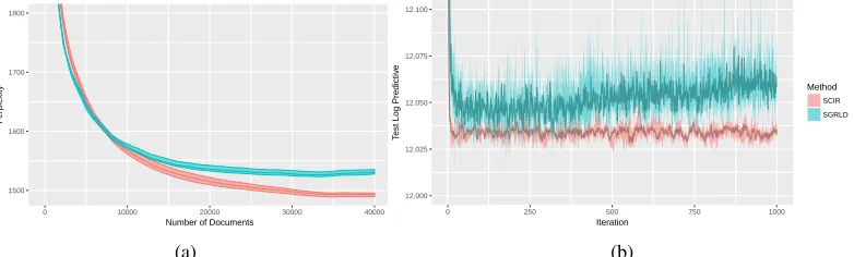
Figure 3: (a) plots the perplexity of SGRLD and SCIR when used to sample from the LDA model of Section 5.1 applied to Wikipedia documents; (b) plots the log predictive on a test set of the anonymous Microsoft user dataset, sampling the mixture model defined in Section 5.2 using SCIR and SGRLD.

iteration a minibatch of 50 documents is sampled in an online manner. We use the same vocabulary set as in Patterson and Teh (2013) which consists of approximately 8000 words. The exponential of the average log-predictive on a held out set of 1000 documents is calculated every 5 iterations to evaluate the model. This quantity is known as the perplexity, and use a document completion approach to calculate it (Wallach et al., 2009). The perplexity is plotted for five runs using different seeds, which gives an idea of variability. Similar to Patterson and Teh (2013), for both methods we use a decreasing stepsize scheme of the formhm=h[1 +m/τ]−κ. The results are plotted in Figure

3a. While the initial convergence rate is similar, SCIR keeps descending past where SGRLD begins to converge. This experiment serves as a good example for the impact that removing the discretization error has for this problem. Further impact would probably be seen if a larger vocabulary size is used, leading to sparser topic vectors. In real-world applications of LDA, it is quite common to use vocabulary sizes above 8000.

5.2 Bayesian Nonparametric Mixture Model

We apply SCIR to sample from a Bayesian nonparametric mixture model of categorical data, based on Dunson and Xing (2009). To the best of our knowledge, the development of SGMCMC methods for Bayesian nonparametric models has not been considered before, so we deem this to be another contribution of the work. In particular, we develop a truncation free, scalable sampler based on SGMCMC for Dirichlet processes (DP, see Ferguson, 1973). For more thorough details of DPs and the stochastic sampler developed, the reader is referred to the Supplementary Material. The model can be expressed as follows

xi|θ, zi∼Multi(ni, θzi), θ, zi ∼DP(Dir(a), α). (5.1) Here Multi(m, φ)is a multinomial distribution withmtrials and associated discrete probability distributionφ; DP(G0, α)is a DP with base distributionG0and concentration parameterα. The DP

component parameters and allocations are denoted byθandzirespectively. We define the number

of observationsN byN :=P

ini, and letLbe the number of instances ofxi,i= 1, . . . , L. This

type of mixture model is commonly used to model the dependence structure of categorical data, such as for genetic or natural language data (Dunson and Xing, 2009). The use of DPs (Ferguson, 1973) means we can account for the fact that we do not know the true dependence structure. DPs allow us to learn the number of mixture components in a penalized way during the inference procedure itself. We apply this model to the anonymous Microsoft user dataset (Breese et al., 1998). This dataset consists of approximatelyN = 105instances ofL= 30000anonymized users. Each instance details part of the website the user visits, which is one ofd= 294categories (hereddenotes the dimension of xi). We use the model to try and characterize the typical usage patterns of the website. Since there are

and SCIR. Once again, we plot runs over 5 seeds to give an idea of variability. The results are plotted in Figure 3b. They show that SCIR consistently converges to a lower log predictive test score, and appears to have lower variance than SGRLD. SGRLD also appears to be producing worse scores as the number of iterations increases. We found that SGRLD had a tendency to propose many more clusters than were required. This is probably due to the asymptotic bias of Proposition 2.1, since this would lead to an inferred model that has a higherαparameter than is set, meaning more clusters would be proposed than are needed. In fact, setting a higherαparameter appeared to alleviate this problem, but led to a worse fit, which is more evidence that this is the case.

6

Discussion

We presented an SGMCMC method, the SCIR algorithm, for simplex spaces. We show that the method has no discretization error and is asymptotically unbiased. Our experiments demonstrate that these properties give the sampler improved performance over other SGMCMC methods for sampling from sparse simplex spaces. Many important large-scale models are sparse, so this is an important contribution. A number of useful theoretical properties for the sampler were derived, including the non-asymptotic variance and moment generating function. Finally, we demonstrate the impact of the sampler on a variety of interesting problems including a novel scalable Dirichlet process sampler. An interesting line of further work would be reducing the non-asymptotic variance, which could be done by means of control variates.

7

Acknowledgments

Jack Baker gratefully acknowledges the support of the EPSRC funded EP/L015692/1 STOR-i Centre for Doctoral Training. Paul Fearnhead was supported by EPSRC grants EP/K014463/1 and EP/R018561/1. Christopher Nemeth acknowledges the support of EPSRC grants EP/S00159X/1 and EP/R01860X/1. Emily Fox acknowledges the support of ONR Grant N00014-15-1-2380 and NSF CAREER Award IIS-1350133.

References

Baker, J., Fearnhead, P., Fox, E. B., and Nemeth, C. (2017). Control variates for stochastic gradient MCMC. Available fromhttps://arxiv.org/abs/1706.05439.

Blackwell, D. and MacQueen, J. B. (1973). Ferguson distributions via polya urn schemes. The Annals of Statistics, 1(2):353–355.

Blei, D. M., Ng, A. Y., and Jordan, M. I. (2003). Latent Dirichlet allocation. Journal of Machine Learning Research, 3:993–1022.

Breese, J. S., Heckerman, D., and Kadie, C. (1998). Empirical analysis of predictive algorithms for collaborative filtering. InProceedings of the Fourteenth Conference on Uncertainty in Artificial Intelligence, pages 43–52.

Chatterji, N. S., Flammarion, N., Ma, Y.-A., Bartlett, P. L., and Jordan, M. I. (2018). On the theory of variance reduction for stochastic gradient Monte Carlo. Available athttps://arxiv.org/abs/ 1802.05431v1.

Chen, T., Fox, E., and Guestrin, C. (2014). Stochastic gradient Hamiltonian Monte Carlo. In Proceedings of the 31st International Conference on Machine Learning, pages 1683–1691. PMLR.

Cox, J. C., Ingersoll, J. E., and Ross, S. A. (1985). A theory of the term structure of interest rates. Econometrica, 53(2):385–407.

Ding, N., Fang, Y., Babbush, R., Chen, C., Skeel, R. D., and Neven, H. (2014). Bayesian sampling using stochastic gradient thermostats. InAdvances in Neural Information Processing Systems 27, pages 3203–3211.

Dunson, D. B. and Xing, C. (2009). Nonparametric Bayes modeling of multivariate categorical data. Journal of the American Statistical Association, 104(487):1042–1051.

Escobar, M. D. and West, M. (1995). Bayesian density estimation and inference using mixtures. Journal of the American Statistical Association, 90(430):577–588.

Ferguson, T. S. (1973). A Bayesian analysis of some nonparametric problems. The Annals of Statistics, 1(2):209–230.

Girolami, M. and Calderhead, B. (2011). Riemann manifold Langevin and Hamiltonian Monte Carlo methods. Journal of the Royal Statistical Society: Series B (Statistical Methodology), 73(2):123–214.

Kalli, M., Griffin, J. E., and Walker, S. G. (2011). Slice sampling mixture models. Statistics and Computing, 21(1):93–105.

Liverani, S., Hastie, D., Azizi, L., Papathomas, M., and Richardson, S. (2015). PReMiuM: An R package for profile regression mixture models using Dirichlet processes. Journal of Statistical Software, 64(7):1–30.

Ma, Y.-A., Chen, T., and Fox, E. (2015). A complete recipe for stochastic gradient MCMC. In Advances in Neural Information Processing Systems, pages 2917–2925.

Nagapetyan, T., Duncan, A., Hasenclever, L., Vollmer, S. J., Szpruch, L., and Zygalakis, K. (2017). The true cost of stochastic gradient Langevin dynamics. Available athttps://arxiv.org/abs/ 1706.02692.

Papaspiliopoulos, O. (2008). A note on posterior sampling from Dirichlet mixture models. Techni-cal Report. Available athttp://wrap.warwick.ac.uk/35493/1/WRAP_papaspliiopoulos_ 08-20wv2.pdf.

Patterson, S. and Teh, Y. W. (2013). Stochastic gradient Riemannian Langevin dynamics on the probability simplex. InAdvances in Neural Information Processing Systems 26, pages 3102–3110.

Rosenblatt, M. (1952). Remarks on a multivariate transformation. The Annals of Mathematical Statistics, 23(3):470–472.

Sato, I. and Nakagawa, H. (2014). Approximation analysis of stochastic gradient Langevin dynamics by using Fokker-Planck equation and Ito process. In Proceedings of the 31st International Conference on Machine Learning, pages 982–990. PMLR.

Sethuraman, J. (1994). A constructive definition of Dirichlet priors.Statistica Sinica, 4(2):639–650.

Teh, Y. W., Thiéry, A. H., and Vollmer, S. J. (2016). Consistency and fluctuations for stochastic gradient Langevin dynamics.Journal of Machine Learning Research, 17(7):1–33.

Vollmer, S. J., Zygalakis, K. C., and Teh, Y. W. (2016). Exploration of the (non-)asymptotic bias and variance of stochastic gradient Langevin dynamics.Journal of Machine Learning Research, 17(159):1–48.

Walker, S. G. (2007). Sampling the Dirichlet mixture model with slices.Communications in Statistics, 36(1):45–54.

Wallach, H. M., Murray, I., Salakhutdinov, R., and Mimno, D. (2009). Evaluation methods for topic models. InProceedings of the 26th Annual International Conference on Machine Learning, pages 1105–1112. PMLR.

Welling, M. and Teh, Y. W. (2011). Bayesian learning via stochastic gradient Langevin dynamics. In Proceedings of the 28th International Conference on Machine Learning, pages 681–688. PMLR.

Wenzhe Li, Sungjin Ahn, M. W. (2016). Scalable MCMC for mixed membership stochastic blockmod-els. InProceedings of the 19th International Conference on Artificial Intelligence and Statistics, pages 723–731. PMLR.

A

Proofs

A.1 Proof of Proposition 2.1

Proof. Define thelocal weak errorof SGLD, starting fromθ0and with stepsizeh, with test function

φby

Eφ(θ1)−φ(¯θh)

,

whereθ¯his the true underlying Langevin diffusion (2.1), run for timehwith starting pointθ0. Then

it is shown by Vollmer et al. (2016) that ifφ:Rd →Ris a smooth test function, and that SGLD

applied with test functionφhas local weak errorO(h), then

E

lim

M→∞1/M

M

X

m=1

φ(θm)−Eπ[φ(θ)]

is alsoO(h). What remains to be checked is that using such a simple function forφ(the identity), does not cause things to disappear such that the local weak error of SGLD is no longerO(h). The identity function is infinitely differentiable, thus is sufficiently smooth. For SGLD, we find that

E[θ1|θ0] =θ0+hf0(θ0).

For the Langevin diffusion, we define the one step expectation using the weak Taylor expansion of Zygalakis (2011), which is valid since we have made Assumptions 3.1 and 3.2 of Vollmer et al. (2016). Define the infinitesimal operatorLof the Langevin diffusion (2.1) by

Lφ=f0(θ)·∂θφ(θ) +∂2θφ(θ).

Then Zygalakis (2011) shows that the weak Taylor expansion of Langevin diffusion (2.1) has the form

E[¯θh|θ0] =θ0+hLφ(θ0) +

h2

2 L

2_{φ(θ0) +O(h}3_).

This means whenφis the identity then

E[¯θh|θ0] =θ0+hf0(θ0) +

h2

2 [f(θ)f

0_{(θ) +f}00_{(θ)] +O(h}3_).

Since the terms agree up toO(h)then it follows that even whenφis the identity, SGLD still has local weak error ofO(h). This completes the proof.

A.2 Proof of Theorem 3.1

Proof. Suppose we have a random variableU∞following a generalized gamma posterior with dataz

and the following density

f(u)∝u2(α+PNi=1zi)−1_e−u2/4_.

Seta:= 2(α+PN

i=1zi), Then∂logf(u) = (2a−1)/u−u/2, so that the Langevin diffusion for

U∞will have the following integral form

Ut+h|Ut=Ut+

Z t+h

t

2a−1

Us

−Us

2

ds+√2

Z t+h

t

dWt.

Applying Ito’s lemma toUtto transform toθt=g−1(Ut) =Ut2/4(hereg(·)has been stated in the

proof), we find that

θt+h|θt=θt+

Z t+h

t

[a−θs]ds+

Z t+h

t

p

2θtdWt.

This is exactly the integral form for the CIR process. This completes the proof.

Now we give more details of the connection between SGLD and SCIR. Let us define an SGLD algorithm that approximately targetsU∞, but without the Euler discretization by

U(m+1)h|Umh=Umh+

Z (m+1)h

mh

_2ˆa

m−1

Us

−Us

2

ds+√2

Z (m+1)h

mh

where aˆm is an unbiased estimate of a; for example, the standard SGLD estimate ˆam = α+

N/nP

i∈Smzi; alsohis a tuning constant which determines how much time is simulated before resamplingˆam.

Again applying Ito’s lemma toUmhto transform toθmh=g(Umh) =Umh2 /4, we find that

θ(m+1)h=θmh+

Z (m+1)h

mh

[ˆam−θs]ds+

Z (m+1)h

mh

p

2θtdWt.

This is exactly the integral form for the update equation of an SCIR process.

Finally, to show SCIR has the desired approximate target, we use some properties of the gamma distribution. Firstly ifθ∞ ∼Gamma(a,1)then4θ∞ ∼Gamma(a,14), so thatU∞= 2

√

θ∞will

have a generalized gamma distribution with density proportional toh(u)∝u2a−1_e−u2_/4

. This is exactly the approximate target of the discretization free SGLD algorithm (A.1) we derived earlier.

A.3 Proof of Theorem 4.1

First let us define the following quantities

r(s) = se

−h

1−s(1−e−h₎, r

(n)_{(s) =r◦ · · · ◦r}

| {z }

n

(s).

Then we will make use of the following Lemmas: Lemma A.1. For alln∈Nands∈R

r(n)(s) = se

−nh

1−s(1−e−nh₎.

Lemma A.2. For alln∈N,s∈R, setr(0)(s) :=s, then

n−1

Y

i=0

h

1−r(i)(s)(1−e−h)i=1−s(1−e−nh).

Both can be proved by induction, which is shown in Section B.

Suppose thatθ1|θ0is a CIR process, starting atθ0and run for timeh. Then we can immediately write

down the MGF ofθ1,Mθ1(s), using the MGF of a non-central chi-squared distribution

Mθ1(s) =E

esθ1_|θ

0

=

1−s(1−e−h)−a

exp

_sθ

0e−h

1−s(1−e−h₎

.

We can use this to find EesθM_|θ

M−1

, and then take expectations of this with respect to

θM−2, i.e. EEesθM|θM−1|θM−2. This is possible because EesθM|θM−1 has the form

C(s) exp[θM−1r(s)], where C(s)is a function only involvings, and r(s)is as defined earlier.

Thus repeatedly applying this and using Lemmas A.1 and A.2 we find

MθM(s) =

1−s(1−e−M h)−aexp

_sθ

0e−M h

1−s(1−e−M h₎

. (A.2)

Although this was already known, we can use the same idea to find the MGF of the SCIR process. The MGF of SCIR immediately follows using the same logic as before, as well as using the form of

MθM(s)and Lemmas A.1 and A.2. Leading to

M_θˆ_M(s) =

M

Y

m=1

h

1−r(m−1)(s)(1−e−h)i

−ˆam

exphθ0r(M)(s)

i

=MθM(s)

M

Y

m=1

_1−s(1−e−mh₎

1−s(1−e−(m−1)h₎

A.4 Proof of Theorem 4.2

Proof. From Theorem 4.1, we have

M_θˆ_M(s) =MθM(s)

M

Y

m=1

1−s(1−e−mh)−(ˆam−a)

| {z }

e0(s)

M

Y

m=1

h

1−s(1−e−(m−1)h)i

−(a−aˆm)

| {z }

e1(s)

.

We clearly haveMθM(0) =e0(0) =e1(0) = 1. Differentiating we find

e0₀(s) =

M

X

i=1

(ˆai−a)(1−e−ih)

1−s(1−e−ih)−1e0(s),

similarly

e01(s) =

M

X

i=1

(a−ˆai)(1−e−(i−1)h)

h

1−s(1−e−(i−1)h)i

−1

e1(s).

It follows that, labeling the minibatch noise up to iterationM byBM, and using the fact thatEaˆi=a

for alli= 1, . . . , Mwe have

EˆˆθM =E

h

E

ˆ

θM|BM

i

=_EhM_ˆ0

θM(0) i

=EMθ0M(0)e0(0)e1(0) +MθM(0)e

0

0(0)e1(0) +MθM(0)e0(0)e

0

1(0)

=EθM.

Now taking second derivatives we find

e00₀(s) =

M

X

i=1

(ˆai−a)(ˆai−a−1)(1−e−ih)2

1−s(1−e−ih)−2

e0(s)

+X

i6=j

(ˆai−a)(ˆaj−a)(1−e−ih)(1−e−jh)

1−s(1−e−ih)−11−s(1−e−jh)−1e0(s).

Now taking expectations with respect to the minibatch noise, noting independence ofˆaiandˆajfor

i6=j,

E[e000(0)] =

M

X

i=1

(1−e−ih)2_Var(ˆai).

By symmetry

E[e001(0)] =

M

X

i=1

(1−e−(i−1)h)2Var(ˆai).

We also have

E[e00(0)e

0

1(0)] =−

M

X

i=1

Now we can calculate the second moment using the MGF as follows, note that E(e00(0)) = E(e01(0)) = 0,

Eθˆ2M =E

h

M_θˆ00_M(0)

i

=EMθ00M(0)e0(0)e1(0) +MθM(0)e

00

0(0)e1(0) +MθM(0)e0(0)e

00

1(0) + 2MθM(0)e

0

0(0)e

0

1(0)

=_Eθ_M2 +

M

X

i=1

(1−e−ih)2_Var(ˆai) + M

X

i=1

(1−e−(i−1)h)2_Var(ˆai)−2 M

X

i=1

(1−e−ih)(1−e−(i−1)h)_Var(ˆai)

=EθM2 +Var(ˆa)

"

e−2M h−1 + 2

M

X

i=1

e−2(i−1)h−e−(2i−1)h

#

=_Eθ_M2 +_Var(ˆa)

"

e−2M h−1 + 2

2M−1

X

i=0

(−1)ie−ih

#

=_Eθ_M2 +_Var(ˆa)

e−2M h−1 + 2−2e

−2M h

1 +e−h

=_Eθ_M2 +_Var(ˆa)(1−e−2M h)

_1−e−h

1 +e−h

B

Proofs of Lemmas

B.1 Proof of Lemma A.1

Proof. We proceed by induction. Clearly the result holds forn= 1. Now assume the result holds for alln≤k, we prove the result forn=k+ 1as follows

r(k+1)(s) =r◦r(k)(s)

=r

_se−kh

1−s(1−e−kh₎

= se

−kh

1−s(1−e−kh₎·

e−h_(1−s(1−e−kh₎₎

1−s(1−e−kh_)−se−kh_(1−e−h₎

= se

−(k+1)h

1−s(1−e−(k+1)h₎.

Thus the result holds for alln∈Nby induction.

B.2 Proof of Lemma A.2

Proof. Once again we proceed by induction. Clearly the result holds forn= 1. Now assume the result holds for alln≤k. Using Lemma A.1, we prove the result forn=k+ 1as follows

k

Y

i=0

h

1−r(i)(s)(1−e−h)i=

1−s(1−e−kh)

1− se

−kh_(1−e−h₎

1−s(1−e−kh₎

=1−s(1−e−kh)

₁

−s(1−e−(k+1)h₎

1−s(1−e−kh₎

=h1−s(1−e−(k+1)h)i

C

CIR Parameter Choice

As mentioned in Section 3, the standard CIR process has more parameters than those presented. The full form for the CIR process is as follows

dθt=b(a−θt)dt+σ

p

θtdWt, (C.1)

wherea,bandσare parameters to be chosen. This leads to a Gamma(2ab/σ2_,2b/σ2_)stationary

distribution. For our purposes, the second parameter of the gamma stationary distribution can be set arbitrarily, thus it is natural to set2b=σ2_{which leads to a Gamma(a,1)stationary distribution and}

a process of the following form

dθt=b(a−θt)dt+

p

2bθtdWt.

Fix the stepsizeh, and use the slight abuse of notation thatθm=θmh. The process has the following

transition density

θm+1|θm=ϑm∼

1−e−bh

2 W, W ∼χ

2

2a,2ϑm

e−bh

1−e−bh

.

Using the MGF of a non-central chi-square distribution we find

MθM(s) =

1−s(1−e−M bh)−a

exp

_sθ

0e−M bh

1−s(1−e−M bh₎

.

Clearlybandhare unidentifiable. Thus we arbitrarily setb= 1.

D

Stochastic Slice Sampler for Dirichlet Processes

D.1 Dirichlet Processes

The Dirichlet process (DP) (Ferguson, 1973) is parameterised by a scale parameterα∈R>0and a

base distributionG0and is denotedDP(G0, α). A formal definition is thatGis distributed according

toDP(G0, α)if for allk∈Nandk-partitions{B1, . . . , Bk}of the space of interestΩ

(G(B1), . . . , G(Bk))∼Dir(αG0(B1), . . . , αG0(Bk)).

More intuitively, suppose we simulateθ1, . . . θN fromG. Then integrating outG(Blackwell and

MacQueen, 1973) we can representθN conditional onθ−N as

θN |θ1, . . . , θN−1∼ 1

N−1 +α

N−1

X

i=1

δθi+

α

N−1 +αG0,

whereδθis the distribution concentrated atθ.

An explicit construction of a DP exists due to Sethuraman (1994), known as the stick-breaking construction. The slice sampler we develop in this section is based on this construction. For

j= 1,2, . . ., setVj∼Beta(1, α)andθj∼G0. Then the stick breaking construction is given by

ωj :=Vj j−1

Y

k=1

(1−Vk) (D.1)

G∼

∞

X

j=1

ωjδθj, (D.2)

and we haveG∼DP(G0, α).

D.2 Slice sampling Dirichlet process mixtures

We focus on sampling from Dirichlet process mixture models defined by

Xi|θi∼F(θi)

θi|G∼G

A popular MCMC algorithm for sampling from this model is theslice sampler, originally developed by Walker (2007) and further developed by Papaspiliopoulos (2008); Kalli et al. (2011). The slice sampler is based directly on the stick-breaking construction (D.2), rather than the sequential (Pólya urn) formulation of (D.1). This makes it a more natural approach to develop a stochastic sampler from; since the stochastic sampler relies on conditional independence assumptions. The slice sampler can be extended to other Bayesian nonparametric models quite naturally, from their corresponding stick breaking construction.

We want to make inference on a Dirichlet process using the stick breaking construction directly. Suppose the mixture distributionF, and the base distributionG0admit densitiesfandg0. Introducing

the variablez, which determines which componentxis currently allocated to, we can write the density as follows

p(x|ω, θ, z)∝ωzf(x|θz).

Theoretically we could now use a Gibbs sampler to sample conditionally fromz,θandω. However this requires updating an infinite number of weights, similarlyzis drawn from a categorical distribu-tion with an infinite number of categories. To get around this Walker (2007) introduces another latent variableu, such that the density is now

p(x|ω, θ, z, u)∝1(u < ωz)f(x|θz),

so that the full likelihood is given by

p(x|ω, θ,z,u)∝

N

Y

i=1

1(ui< ωzi)f(xi|θzi). (D.3)

Walker (2007) shows that in order for a standard Gibbs sampler to be valid given (D.3), the number of weightsωjthat needs to be sampled given this new latent variable is now finite, and given byk∗,

wherek∗is the smallest value such thatPk∗

j=1ωj>1−ui.

The Gibbs algorithm can now be stated as follows, note we have included an improvement suggested by Papaspiliopoulos (2008), in how to samplevj.

• Sample the slice variablesu, given byui |ω,z∼U(0, ωzi)fori= 1, . . . , N. Calculate

u∗= minu.

• Delete or add components until the number of current componentsk∗is the smallest value such thatu∗<1−Pk∗

j=1ωj.

• Draw new component allocationszifori= 1, . . . , N, using

p(zi=j|xi, ui, ω, θ)∝1(ωj> ui)f(xi|θ).

• Forj≤k∗, sample new component parametersθjfrom

p(θj|x,z)∝g0(θj)Q_i:zi=jf(xi|θj)

• Forj≤k∗_{calculate simulate new stick breaksvfrom}

vj|z, α∼Beta

1 +mj, α+Pk

∗

l=j+1ml

. Heremj:=PN_i=11zi=j.

• Updateωusing the newv:ωj=vjQl<j(1−vj).

D.3 Stochastic Sampler

The conditional independence of each update of the slice sampler introduced in Section D.2 makes it possible to adapt it to a stochastic variant. Suppose we updateθandvgiven a minibatch of the zanduparameters. Then since thezanduparameters are just updated from the marginal of the posterior, only updating a minibatch of these parameters at a time would leave the posterior as the invariant distribution. Our exact MCMC procedure is similar to that in theRpackagePReMiuM (Liverani et al., 2015), though they do not use a stochastic sampler. First define the following:

Z∗= maxz;S⊂ {1, . . . , N}is the current minibatch;u∗= minuS;k∗is the smallest value such

thatPk∗

j=1ωj >1−u∗. Then our updates proceed as follows:

• Forj= 1, . . . , Z∗samplevjstochastically with SCIR from

vj|z, α∼Beta(1 + ˆmj, α+P

k∗

l=j+1mˆl). Heremˆj=N/nPi∈S1zi=j. • Updateωjusing the newv:ωj =vjQl<j(1−vj).

• Forj= 1, . . . , Z∗sampleθjstochastically with SGMCMC from

p(θj|x,z)∝g0(θj)Q_Sjf(xi|θj). HereSj={i:zi=jandi∈S}.

• Fori∈Ssample the slice variablesui|ω,z∼U(0, ωzi).

• Sampleαif required. Using Escobar and West (1995), for our example we assume a Gamma(b1, b2)prior so thatα|v1:Z∗∼Gamma(b₁+Z∗, b₂−PK

∗

j=1log(1−vj)).

• Recalculateu∗. Sample additionalωj from the prior, untilk∗is reached. Forj = (Z∗+

1), . . . , k∗sample additionalθjfrom the prior.

• Fori∈S, samplezi, whereP(zi=j|ui, ω, θ,x)∝1(ωj> ui)f(xi|θj).

Note that for our particular example, we have the following conditional update for θ(ignoring minibatching for simplicity):

θj|zj,x∼Dirichlet

 a+

X

i∈Sj

xi1, . . . , a+

X

i∈Sj

xid

 .

E

Experiments

E.1 Synthetic

We now fully explain the distance measure used in the synthetic experiments. Suppose we have random variablesX taking values inRwith cumulative density function (CDF)F. We also have

an approximate sample fromX,Xˆ with empirical density functionFˆ. The Kolmogorov-Smirnov distancedKSbetweenXandXˆis defined bydKS(X,Xˆ) = supx∈R

ˆ

F(x)−F(x)

.However the Dirichlet distribution is multi-dimensional, so we measure the average Kolmogorov-Smirnov distance across dimensions by using the Rosenblatt transform (Rosenblatt, 1952).

Suppose now that X takes values in Rd. Define the conditional CDF of Xk = xk|Xk−1 =

xk−1, . . . , X1 = x1 to beF(xk|x1:(k−1)). Suppose we have an approximate sample from X,

which we denotex(m)_{, form= 1, . . . M. DefineF}ˆ

jto be the empirical CDF defined by the

sam-plesF(x(_jm)|x_1:((m_j)₋₁₎). Then Rosenblatt (1952) showed that ifXˆ is a true sample fromXthenFˆj

should be the uniform distribution and independent ofFˆk fork 6= j. This allows us to define a

Kolmogorov-Smirnov distance measure across multiple dimensions as follows

dKS(X,Xˆ) =

1

K

K

X

j=1 sup

x∈R

ˆ

Fj(x)−Fj(x)

.

Where here applying Rosenblatt (1952),Fj(X)is just the uniform distribution.

The full posterior distributions for the sparse and dense experiments are as follows:

ωsparse|z∼Dir[800.1,100.1,100.1,0.1,0.1,0.1,0.1,0.1,0.1,0.1],

ωdense|z∼Dir[112.1,119.1,92.1,98.1,95.1,96.1,102.1,92.1,91.1,103.1].

For each of the five random seeds, we pick the stepsize giving the bestdKSfor SGRLD and SCIR

from the following options:

Method h

SCIR 1.0 5e-1 1e-1 5e-2 1e-2 5e-3 1e-3 SGRLD 5e-1 1e-1 5e-2 1e-2 5e-3 1e-3 5e-4 1e-4

E.2 Latent Dirichlet Allocation

As mentioned in the main body, we use a decreasing stepsize scheme of the formhm=h(1+m/τ)−κ.

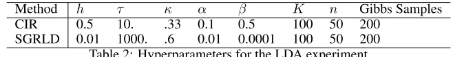
We do this to be fair to SGRLD, where the best performance is found by using this decreasing scheme (Patterson and Teh, 2013; Ma et al., 2015); and this will probably reduce some of the bias due to the stepsizeh. We find a decreasing stepsize scheme of this form also benefits SCIR, so we use it as well. Notice that we find similar optimal hyperparameters for SGRLD to Patterson and Teh (2013). Table 2 fully details the hyperparameter settings we use for the LDA experiment.

Method h τ κ α β K n Gibbs Samples

CIR 0.5 10. .33 0.1 0.5 100 50 200

SGRLD 0.01 1000. .6 0.01 0.0001 100 50 200 Table 2: Hyperparameters for the LDA experiment

E.3 Bayesian Nonparametric Mixture

For details of the stochastic slice sampler we use, please refer to Section D. Figure 3 details full hy-perparameter settings for the Bayesian nonparametric mixture experiment. Note thathθcorresponds

to the stepsizes assigned for sampling theθparameters; whilehDP corresponds to the stepsizes

assigned for sampling from the weightsωfor the Dirichlet process.

Method hθ hDP a K n

CIR 0.1 0.1 0.5 20 1000

SGRLD 0.001 0.005 0.001 30 1000