An Inventory Model for Items with Two Parameter Weibull Distribution Deterioration and Backlogging

(1)

An Inventory Model for Items with Two Parameter

Weibull Distribution Deterioration and Backlogging

Nandagopal Rajeswari, Thirumalaisamy Vanjikkodi Sri GVG Visalakshi College for Women, Udumalpet, India

Email: Rajinand63@rediffmail.com

Received February 3, 2012; revised March 11, 2012; accepted March 22, 2012

ABSTRACT

In this paper an inventory model is developed with time dependent power pattern demand and shortages due to deterioration and demand. The deterioration is assumed to follow a two parameter Weibull distribution. Three different cases with complete, partial, no backlogging are considered. The optimal analytical solution of the model is derived. Suit-able numerical example has been discussed to understand the problem. Further sensitivity analysis of the decision variables has been done to examine the effect of changes in the values of the parameters on the optimal inventory policy.

Keywords: Inventory; Weibull Deterioration; Shortages; Power Demand; Partial Backlogging; Complete Backlogging

1. Introduction

Deterioration of items in an inventory is a common phe- nomenon in business situations. This is due to the fact that the items in the inventory become obsolete, devalued, decay or damaged depending on the type of goods. As a consequence of the deterioration shortages may occur. Hence deterioration factor has to be given importance while determining the optimal policy for an inventory model.

Whitin [1] was the first to consider the deterioration of inventory items, he dealt with the deterioration of fashion goods at the end of prescribed storage period. Ghare and Schrader [2] later formulated a mathematical model with a constant deterioration rate. Covert and Philip [3] then extended Ghare and Schrader’s model for variable rate of deterioration by assuming two parameter Weibull distribution functions.

Resently, researchers are analyzing the effect of deterioration and the variations in the demand rate with time in supply chain and logistics. Dave and Patel [4] derived a lot size model for constant deterioration of items with time proportional demand. Sachan [5] modified Dave and Patel’s [4] model. Goel and Aggarwal [6] formulated an order-level inventory system with power-demand pattern for deteriorating items. Datta and Pal [7] presented an EOQ model with the demand rate dependent on in- stantaneous stock displayed until a predefined maximum level of inventory L is achieved. After this level is re-

ached, the demand rate becomes constant (D(t) = a[I(t)b_]

for I(t) > L and D(t) = aLb_{for 0}_ _I₍_t₎_ _L_{). Chang and}

Dye [8] developed an EOQ model with a similar power demand and considered partial backlogging of orders. He stated that if longer the waiting time smaller the backlogging rate would be. So the proportion of the customers who would like to accept backlogging at time tde- creases with the waiting time for the next replenishment. In this situation the backlogging rate is defined as



1



( )

1 i

B t

t t

 

  (1.1)

where tiis the time at which the ithreplenishment is being

made and δ is the backlogging parameter. Several researchers have extended their idea to different situations con- sidering various deterioration rates and time value of money. Valuable models in this direction are the models of S. R. Singh, and T. J. Singh [9], Tarun Jeet Singh, Shiv Raj Singh and Rajul Dutt [10], C. K. Tripathy and L. M. Pradhan [11], etc.

(2)

[image:2.595.54.287.102.277.2]

Table 1. Variations in parameters “α” and “”.

Parameter

value % Change t1 (Year) Q (Units) K1 ($)

–50 0.489700 50.001118 770.07

–25 0.489652 50.001675 770.07

0 0.489604 50.002235 770.08

+25 0.489556 50.002792 770.08

α

+50 0.489508 50.003349 770.09

–50 0.488999 50.016720 770.19

–25 0.489404 50.005856 770.11

0 0.489604 50.002235 770.08

+25 0.489702 50.000896 770.06



[image:2.595.56.284.309.541.2]

+50 0.489750 50.000370 770.06

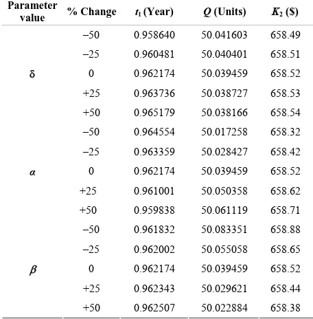
Table 2. Variations in parameters “”, “α” and “”.

Parameter

value % Change t1 (Year) Q (Units) K2 ($) –50 0.958640 50.041603 658.49 –25 0.960481 50.040401 658.51 0 0.962174 50.039459 658.52 +25 0.963736 50.038727 658.53 

+50 0.965179 50.038166 658.54 –50 0.964554 50.017258 658.32 –25 0.963359 50.028427 658.42 0 0.962174 50.039459 658.52

+25 0.961001 50.050358 658.62

α

+50 0.959838 50.061119 658.71 –50 0.961832 50.083351 658.88

–25 0.962002 50.055058 658.65 0 0.962174 50.039459 658.52 +25 0.962343 50.029621 658.44



+50 0.962507 50.022884 658.38

Table 3. Variations in parameters “α” and “”.

Parameter

value % Change t1 (Year) Q3 (Units) K3 ($)

–50 0.979287 50.014481 658.42

–25 0.978537 50.026192 658.53

0 0.977791 50.037792 658.63 +25 0.977048 50.049282 658.74

α

+50 0.976309 50.060665 658.84 –50 0.977678 50.081963 658.99 –25 0.977732 50.053524 658.76

0 0.977791 50.037792 658.63 +25 0.977851 50.027828 658.55



+50 0.977912 50.020977 658.49

2. Notations and Assumptions

2.1. Notations

A: The ordering cost per inventory cycle. C: The purchase cost per unit.

H: The inventory holding cost per unit per time unit.

b: The backordered cost per unit short per time unit. l: The cost of lost sales per unit.

t1: The time at which the inventory level reaches zero, t1 0.

t2: The length of period during which shortages are al-lowed, t2  0.

T: (= t1 + t2) The length of cycle time.

Im: The maximum inventory level during [0, T].

Ib: The maximum backordered units during stock out

period.

Qi: (= Im + Ib) The order quantity in cycle of length T

corresponding to no backlogging, partial backlogging and complete backlogging).

I1(t): The level of positive inventory at time t, 0  t t1.

I2(t): The level of negative inventory at time t, t1t T.

Ki: The total cost per time unit.

2.2. Assumptions

 The inventory consists of only one type of items.

(1n n)/  The expression for demand rate is dt _1/_n

nT at any

time t, where d is a positive constant, n may be any positive number, T is the planning horizon.

 The variable deterioration rate (t) is assumed to follow the two parameter weibull distribution function (i.e.) (t) = αβtβ1_{, where}_α_{is the scale parameter,}_α_> 0; β is the shape parameter β > 0; t is the time to deterioration, t > 0. The replenishment rate is infinite.

 The lead-time is zero or negligible.

 The planning horizon is infinite.

 During the stock out period, the backlogging rate is variable and is dependent on the length of the waiting time for the next replenishment. The proportion of the customers who would like to accept the backlogging at time “t” is with the waiting time (T  t) for the next replenishment i.e., for the negative inventory the backlogging rate is ( ) 1

1 ( )

B t

T t

 

  ;  > 0 denotes

the backlogging parameter and t1  t  T.

3. Mathematical Model

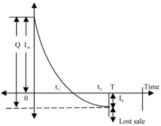
[image:2.595.56.284.569.735.2]

(3)

[image:3.595.91.254.83.211.2]

Figure 1. Representation of inventory system. 3.1. Inventory Level before Shortage Period During the period [0, t1], the inventory depletes due to the demand and deterioration. Hence, the differential equation governing the inventory level I1(t) at any time t during the cycle [0, t1] is given by

1

1 1 ,0 1

n n

n

t t



  

1 1

d ( )

( ) d

I t _t _{I t} dt

t

nT



 

  (3.1)

with the boundary condition I1(t1) = 0 at t = t1. The solution of Equation (3.1) is given by

1

1 1

1

( )

(1 )

1

0

n n

n I t

d _t _t _t

n T

t t

 





 

  _  _



 

 

1 1

1

n n

t t

 

 

  



 _ _

  

  (3.2)

The maximum positive inventory level is

1 1

1

1 1

1

n n

n t

t

n

  1

(0)

MI

n d

I I

T 



 

 _ 

 

 

  (3.3)

3.1.1. Model I: (No Backlogging)

The state of inventory during the shortage period [t1,T] is represented by the differential equation,

1 2

d ( ) d

I t dt

t

nT

  ₁ ,₁

n n

n

t t T



  (3.4)

1 1

1 ,1

n n

2( ) 1

n

d

I t t

T

  _ t _ t  t T

  (3.5)

The maximum backordered units are 1 1

2 1 n 1n

n

d ( )

MB

I  I T 

Hence, the order size during [0,T] is Q1 = IMI + IMB.

T t

T

 



 

  (3.6)

1 1

1

1 1 ₁

n n n n

t d

Q T

n T

 

  





 _  _ (3.7)



 

 

OC

3.1.1.1. Cost Components

The total cost per replenishment cycle consists of the following cost components.

3.1.1.2. Ordering Cost per Cycle (IOC)

I A (3.8)

3.1.1.3. Inventory Holding Cost per Cycle (IHC)

1

1 0

1 1

1

( )d

1 ( 1)(1 )

t HC

n n n

n n

n

I h I t t

t t

hd

n n n

T

 

 

  



 

 

 _  _

   

 

 







(3.9)

3.1.1.4. Backordered Cost per Cycle (IBC)

1

2

1 1

1 1 1 1

π ( ) d

π

1 1

T

BC b

t

n n

b n

n

I I t t

d nT nt

Tt

n n

T

 

 

 

 

 _   _

 

 

 



(3.10)

3.1.1.5. Purchase Cost per Cycle (IPC) 1 1

1

1 1 ₁

n n n PC

n

t Cd

I C Q T

n T

 





 

 

   _  _



 

 

(3.11)

Hence, the total cost per time unit from (3.8), (3.9), (3.10), (3.11) is





1 1

OC HC BC LS PC

K I I I I I

T

     (3.12) To minimize total average cost per unit time (K1), the optimal value of t1can be obtained by solving the equa-tion

1

1 d

0 d

K

t  (3.13)

The value of t1 obtained from (3.13) is used to obtain the optimal values of Q1 and K1. Since the Equation (3.13) is nonlinear, it is solved using MATLAB.

The condition 2

1 2 1 d

0 d

K

(4)

3.1.2. Model II: (Partial Backlogging)

3.1.2.1. Inventory Level during Shortage Period

During the interval [t1,T] stock out situation arises. The orders during this period are partially backlogged. The state of inventory during [t1,T] can be represented by the differential equation, 1 1 , ( ) n

t t T

t            _{ } 1 2 d ( )

d 1 n n dt nT I t

t    T (3.15)

2 1 1 1 1 (1 ) 1 n n n d

T t t

n T

t t T

       _  _      1 1 1 1 ( ) n n n n I t t t        _ _   

  (3.16)

The maximum backordered units are 2

1 (1 )

1 MB n d T n         1 1 1 1 1 1 ( ) n n n n n n

I I T

T T t

T t                   _  _   2 (3.17)

Hence, the order size during [0,T] is Q IMI IMB .

2 1 1 1 1 1 1 n n n n d _t T n T Tt n n          _  _ 

 ₁1n 1nn ₁1nn

Q T t   _          _ __ (3.18)

3.1.2.3. Backordered Cost per Cycle (IBC )









1 2 1 1 2 1 1 1 2 1 2 2 1

π ( ) d

π

2

(1 )(1 2 ) 1 2

BC b t n n b n n n n n n

I I t t

d _nT t T T T t n T n n             _ _       



1 1

(1 2 )

1 1 T n n T t n n n         (3.19)

3.1.2.4. Cost Due to Lost Sales per Cycle (ILS)

1 1 1 1 1 1 1 1 1 1

π 1 d

1 ( )

π 1 1 n T _n LS l t n n n n n l n n dt _t T t nT

d nT _Tt t

n n T         _{ }   _  _{ } _     _ _      _   _      



(3.20) I

3.1.2.5. Purchase Cost per Cycle (I_PC ) 2

1

1 1 1 1

1

1 1

1 ₁ ₁

PC

n

n n

n

n n n

n

I C Q

t

Cd _T _Tt _nT

n n T   _          n t     _   _    _ __  _{ } _     (3.21) Hence, the total cost per time unit from (3.8), (3.9), (3.19), (3.20), (3.21) is





2 OC HC BC LS PC

1

K I I I I I

T  

     (3.22) To minimize total average cost per unit time (K2), the optimal value of t1can be obtained by solving the equ -tion

a

2

dK _₀

d from (3.23) is used to obtain the optimal values of Q2 and K2. Since the Equation (3.23) is nonlinear, it is solved using MATLAB.

1 dt The value of t1 obtaine

(3.23)

The condition 2 d K

3.1.3. Model III: (Complete Bac

3.1.3.1. Inventory Level during Shortage Period D

esented by the differential equation,

2 2 1

0

dt  , is also satisfied for the value t1 from (3.23). (3.24)

klogging)

uring the interval [t1,T] stock out situation arises. the orders during this period are completely backlogged. The state of inventory during [t1,T] can be repr

1n

1 n dt     2 d ( )

,

d 1 ( )

nT I t

t T t

 

 

 

1 t  t T

n

 

 

(3.25)

(5)

2( )

I t

1 1 1 1

1 1 1 1 1 (1 ) 1 n n

n n n n

n

d

T t t t t

n T

t t T

           _  _ _  _           (3.26)

The maximum backordered units are

2

1 1 1 1

1 n _nn

d      

1 1

1 (1 T T) n tn ₁ _n T n t

   _  _ _        ( ) MB n

I I T

T           (3.27)

Hence, the order size during [0,T] is Q₃I_MI I_M_B. 3 1 1 1 1 1 1 1 1 n n n n

n n n n

Q

t d

T Tt nT t

                 __  (3.28)

3.1.

1

1 ₁ ₁

n n n

T      _

3.3. Backordered Cost per Cycle (I_BC )





1 2 1 1 2 1 1 1 1

π ( ) d

π _{(1 2 )}

( )

1 1

) 1 2

T BC b t n n n n b n

I I t t

d _nT _{T t}

T T t

n n n          _ _ _  _ _  _  _



(3.29) cle ( 1 2 2 1 2

(1 )(1 2

n n n n _t n T n n  _     1 2 n T  

3.1.3.4. Cost Due to Lost Sales per Cy I_LS )

1 1 1 1 1 π 1 1 ( π T LS l t n n l n 1 1 1 1 1 d ) 1 1 n n n n n n dt I t nT t n n      _{ }   _{ } _   _ _     _ _     

3.1.3.5. Purchase Cost per Cycle (

T t d nT Tt T          



(3.30) PC

I )

3 1 1 1 1 1 1 1 1 n n n n n 1 1 1 1 PC n n n n C Q t Cd

T Tt nT t

n n T          _ _    _    _  __  _{ } _     (3.31)

Hence, the total cost per time unit from (3.8), (3.9),

(3.29), (3.30), (3.31) is

I





3 1

OC HC BC LS PC

K I I I I I

T   

     (3.32)

To minimize total average cost per unit 3 optimal value of t1can be obtained by solving the equa-tion

time (K), the

3 d

0

K _

(3.33)

The value of t1 obtained from (3.33) is used to obtain the optimal values of Q3 and K3. Since the Equat

is nonlinear, it is solved using MATLAB. The condition 1 dt ion (3.33) 2 3 2 1 d 0 d K

t  , is also satisfied for the value t1 from (3.33). (3.34)

wing section. Sensitivity analysis is carried out with respect to backlogging

and deterioration rate.

alysis

In this section the optimal value ( quantity (Qi

To illustrate and validate the proposed model, appro- priate numerical data is considered and the optimal values are found in the follo

parameter

4. Numerical Example and Sensitivity

An

1

t_{), the optimal order} _{) and the minimum to}

i

tal average cost (K) ar

l 0.04 units, α =

0.

its. This advices the retailer to (by

i

e computed for the data given below:

d = 50 units, n = 2 units, T = 1 year, A = $ 250 per order, C = $ 8.0 per unit, h = $ 0.50 per unit per year, b = $ 12.0 per unit per year, = $ 15.0 per unit,  =

01,  = 4.

4.1. Optimum Solution 4.1.1. Model I

For the above numerical values, when deterioration rate is 5%, the optimum time t1 at which positive inventory is zero is 0.489604 time units and stock out period t2 is of length is 0.510396 time un

buy 50 units which will cost a minimum of $ 770.06 rounding off Q_).

The following observations have been made on the ba- p

nventory period,

in order quantity and decrease in total cost per time unit.

ange in the parameters α, β

a marginal change in total cost per time sis of the above table with the increase in scale parameter (α) and sha e parameter (β):

 Increase in α results in decrease in i

increase in order quantity and increase in total cost per time unit.

 Increase in β results in increase in inventory period, decrease

Hence in general 50% ch results only in

(6)

h will cost a minimum of $ 658.20 (by ro

e increase in backlogging

only in a marginal change in total cost per tim

en licy based on general Weibull pattern In

1 is used. Similarly n = 1 and n =

backlogging, partial backlogging and co

to be strictly convex. Sensitivity analysis has been carried out with the change in parameters. The total cost

with backlogging of orders. 4.1.2. Model II

For the above numerical values, when deterioration rate is 5%, the optimum time t1 at which positive inventory is zero is 0.962174 time units and stock out period t2 is of length is 0.037826 time units. This advices the retailer to buy 50 units w ich

mand respectively. Focusing on this concept the optimal order quantity has been computed, for three different cases namely, no

mplete backlogging, by minimizing the total inventory cost and the minimized objective cost function is ob- served

unding off Qi*).

The following observations have been made on the ba- sis of the above table with th

is seen to decrease parameter, scale parameter and shape parameter:

 Increase in δ results in increase in inventory period, decrease in order quantity and increase in total cost

REFERENCES

[1] G. Hadley and T. M. Whitin, “Analysis of Inventory Sys-tems,” Prentice-Hall, New Jersey, 1963.

[2] P. M. Ghare and G. F. Schrader, “A Model for an Expo-nentially Decaying Inventory,” Journal of Industrial En-gineering, Vol. 14, 1963, pp. 238-243.

[3] R. P. Covert and G. C. Philip, “An EOQ Model for Dete-riorating Items with Weibull Distributions Deterioration,”

AIIE Transactions, Vol. 5, No. 4, 1973, pp. 323-332. doi:10.1080/05695557308974918

[4] U. Dave and L. K. Patel, “(T, Si) Policy Inventory Model for Deteriorating Items with Time Proportional Demand,”

Journal of the Operational Research Society, Vol. 32, 1981, pp. 137-142.

[5] R. S. Sachan, “On (T, Si) Policy Inventory M per time unit.

 Increase in αresults in decrease in inventory period, increase in order quantity and increase in total cost per time unit.

 Increase in β results in increase in inventory period, decrease in order quantity and decrease in total cost per time unit.

Hence in general 50% change in the parameters δ, α, β

results only in a marginal change in total cost per time unit.

4.1.3. Model III

For the above numerical values, when deterioration rate is 5%

odel for Deteriorating Items with Time Proportional Demand,”

Journal of the O , Vol. 35, No.

11, 1984, pp. 1 , the optimum time t1 at which positive inventory is

zero is 0.969997 time units and stock out period t2 is of length is 0.030003 time units. This advices the retailer to

y

perational Research Society

013-1019.

[6] V. P. Goel and S. P. Aggarwal, “Order Level Inventory System with Power Demand Pattern for Deteriorating bu 50 units which will cost a minimum of $ 658.28 (by

rounding off Qi

_).

The following observations have been made on the ba-

Items,” Proceedings of the All India Seminar on Opera-tional Research and Decision Making, University of Delhi, New Delhi, 1981, pp. 19-34.

sis of the above table with the increase in scale parameter and shape parameter:

 Increase in α results in decrease in inventory period,

[7] T. K. Datta and A. K. Pal, “Order Level Inventory System with Power Demand Pattern for Items with Variable Rate of Deterioration,” Indian Journal of Pure and Applied Mathematics, Vol. 19, No. 11, 1988, pp. 1043-1053. increase in order quantity and increase in total cost

per time unit.

 Increase in β results in increase in inventory period, [8] H. J. Chang and C. Y. Dye, “An EOQ Model for Dete-_{riorating Items with Time Varying Demand and Partial} Backlogging,” Journal of the Operational Research Soci-ety, Vol. 50, No. 11, 1999, pp. 1176-1182.

decrease in order quantity and decrease in total cost per time unit.

Hence in general 50% change in the parameters α, β

results [9] S. R. Singh and T. J. Singh, “An EOQ Inventory Model _{with Weibull Distribution Deterioration, Ramp Type De-} mand and Partial Backlogging,” Indian Journal of Mathe- matics and Mathematical Sciences, Vol. 3, No. 2, 2007, pp. 127-137.

e unit.

5. Conclusion

In this paper, we have developed a deterministic invent- tory model with power pattern demand and Weibull deterioration rate. This type of power pattern demand re- quires a differ t po

[10] T. J. Singh, S. R. Singh and R. Dutt, “An EOQ Model for Perishable Items with Power Demand and Partial Back-logging,” International Journal of Production Economics, Vol. 15, No. 1, 2009, pp. 65-72.

. _[11]_{C. K. Tripathy and L. M. Pradhan, “An EOQ Model for} Weibull Deteriorating Items with Power Demand and Partial Backlogging,” International Journal of Contem-porary Mathematical Sciences, Vol. 5, No. 38, 2010, pp. 1895-1904.

cases when large portion of demand occurs at the be- ginning of the period n > 1 will be used and when it is large at the end 0 < n <