Increasing cancer cell recognition with Raman microscopic data using sparse coding

July 3, 2018

BACHELOR THESIS−APPLIED MATHEMATICS

INCREASING CANCER

CELL

RECOGNITION

WITH RAMAN

MICRO-SCOPIC DATA USING

SPARSE CODING

Pascal Loohuis

Faculty of Electrical Engineering, Mathematics and Computer Science (EEMCS) Applied Analysis

Increasing cancer cell recognition with

Raman microscopic data using sparse

coding

P. Loohuis

3rd July 2018

Abstract

Traditional methods of research on cancer cells are done via tissue biopsy. Due to the fact that these biopsies are poorly able to predict the treatment response, other research methods are investigated to eventually replace tissue biopsies. One method is performing research on circulat-ing tumor cells from the blood stream, whereas Raman microscopic tech-niques are used to distinguish different sorts of cancer. This data is used to obtain a fingerprint per sort cancer by classifying the data. Principle component analysis (PCA) is used in order to make this hyperspectral data insightful. Data often contains nonlinear statistical dependencies, so it is questionable if PCA is the right method to use. This report introduces two other methods, based on sparse coding, that tackles this shortcom-ing of PCA. In sparse codshortcom-ing a signal is decomposed in a multiplication between a set of basis vectors and a sparse matrix, whereas each pixel of the hyperspectral data will be described with only a few of these basis vectors. The introduced methods proved to give good classifications and were noise resilient.

Keywords —sparse coding, PCA, cancer cells, hyperspectral imaging, Raman ISTA, CoD

*_{Student Applied Mathematics, S1725866, University of Twente, Enschede, the Netherlands.}

1

Introduction

A

compos-ition of cancer cells is therefore an important topic within the health-care community these days. Current cancer diagnostics is primarily done via tis-sue biopsy. A single biopsy has shown its limitations due to the heterogeneity of the tumor. Although multiple biopsies sounds like a clear continuation, the implementation is rather impractical because of its invasive nature and risks[15]. Acquisition of cancer tissue is necessary for cancer research so re-searchers have been searching for other ways to gain cancer cells. Circulating tumor cells(CTCs) in the blood vessels have been chosen as an alternative be-cause the isolation of these cells is safe and less expensive[25]. Identification of the composition of these cells can be done via Raman microscopy. Raman microspectroscopy is an imaging technique that uses hyperspectral cameras to measure the electromagnetic energy scattered from a sample using laser excitation. These energy characteristics are measured in thousands of spec-tral bands and are then used to obtain a fingerprint from cells based on their scattered light[11, 17]. The fingerprint will serve as an input for unsuper-vised statistical classification methods like hierarchical cluster analysis (HCA) andprincipal component analysis(PCA). Use of the latter clusters the different cell components such that distinction between them can be visualized and different cell types can be classified.

Processing the hyperspectral data, compared to classical fluorescent images, leads to a great increase in the processing complexity and time. Therefore, effectively reducing the amount of data is an essential task for hyperspectral data analysis. One common approach for this dimensionality reduction is PCA. It is a type of dimensionality reduction where high dimensional data will be expressed in a lower dimensional dataset of active components. PCA tries to select a few mutually independent principle components which de-scribes the data set best and uses all components to represent each pixel of the observed data [11, 13, 26].

Although PCA is frequently used, there are some drawbacks to this method. Due to the fact that the principal components have to be orthogonal, the method is less flexible[24]. Furthermore, PCA is a good method for data where linear pairwise correlations are predominate, but data often contains important higher-order statistical dependencies. If so, then it is questionable if PCA is the right way to go[18].

learned dictionary. A dictionary learning algorithm from [24] will be used in this paper because of its fast convergence.

2

Background information

Cancer tissue has been important for cancer diagnosis, the cancer’s fingerprint and the prediction of matching cancer therapy. Until now, there has been no evidence that increasing the understanding of the tumor via tissue biopsies has led to an increase in treatment response or even survival. The heterogen-eity of cancer cells and its dynamic characteristics over time are responsible for this poor prognosis. Research has shown that one biopsy is inadequate to map the full diversity of the cancer and even multiple biopsies are not appropriate for this task, because multiple biopsies do not provide enough information and are impractical due to clinical risks for the patient[16].

Because a good identification of the tumor is essential for an optimal treat-ment [9, 21], researchers have been searching for other methods to gain cancer cells for research. CTCs have become an attractive alternative for obtaining tumor tissue because the described disadvantages do not occur. So-called "li-quid biopsy" can be used for the accession of cell-free DNA from cancer cells and the CTCs. These cells are released in the blood vessels during the spread of the cancer. This method of obtaining cancer cells has the advantage that taking multiple samples do not harm the patient and the segregating of pure cancer tissue and other material is not expensive and difficult[21].

Mapping the characteristics of these cells can be done in different ways. Pop-ular methods make use of microscopic equipment, e.g. CellSearch®.Scanning Electron Micropscopy (SEM) and Raman micro-spectroscopy are microscopic techniques for revealing the characteristics of cancer tissue. SEM uses beams of electrons to gain information about the sample’s surface morphology. The fact that it makes use of electron beams ensures high resolution data from the sample’s surface. Raman microscopy uses laser excitation on the sample and collects the scattered light from the tissue. This scattered light can be used for the classification of cell composition but is less accurate than SEM because laser beams are substantially bigger than electrons. In figure 1a and 1b below the results of cell measurements from both methods are shown. For the rest of the report the focus will lie on Raman data.

(a)SEM images of several cancer cells.

(b)A Raman image of a cell with corresponding pixel characteristics.

(c)Results of HCA performed on preprocessed Raman data of the cells in figure 1a.

3

PCA analysis for hyperspectral images

In this section an overview is given of the current method for cancer cell re-cognition. This section contains a short description of all preprocessing steps, an overview of the PCA algorithm and a brief description of the clustering method.

3.1

Preprocessing

Before PCA is performed, preprocessing techniques are applied on the Raman data. Below, all the preprocessing steps performed on the raw data are given in order[17]:

(i) cosmic rays and outliers are removed;

(ii) the region of interest is divided in cell or background. The area outside this region will not be included;

(iii) the solvent residue of the sample is subtracted by using a linear least squares fit; and

(iv) furthermore, a baseline correction an denoising is executed.

3.2

PCA

3.2.1 Principle components

When the preprocessing is done, the PCA algorithm can be used as a di-mensionality reduction tool. The main reasons why this algorithm is used is because of its power to make data insightful and its low computational costs. Suppose this method is used on data containingkpixels with each containing

nspectral bands, we have the following data matrix of dimensionn x k:

X=



   

X11 X12 · · · X1k X21 X22 · · · X2k

..

. ... . .. ...

Xn1 Xn2 · · · Xnk 

   

The goal of PCA is to find a m−dimensional subspace (i.e. m < k), while maintaining the utmost of the variation in the data. The new measurements

W1, . . . ,Wk are linear combinations of the column of X, so each Wp (p = 1, . . . ,k)can be expressed as follows.

Wp=c1pX1+c2pX2+· · ·+c1pXp

where cTp = (c1p,c2p, . . . ,ckp) are constants and cov(Wi,Wj) = 0 for i 6= j. The last constraint ensures the new measurements to be orthogonal[2].

(a)Orginal data.

(b)Calculation the principle components.

(c)Switch the axis.

Figure 2: Schematisation construction principle components[4].

The calculatedWp(p=1, . . . ,k)are called the principle components(PCs). There is no standard number of PC that need to be calculated but at least a 80% coverage of the variation is suggested[2]. The first PC represents the direction with the biggest vari-ation. The next PC will be ortho-gonal (because the covariance with the first PC is equal to zero) and rep-resents the direction with the second largest variation. The remainder components are calculated in a sim-ilar way.

The calculated PCs helps to make the data insightful. The process needed is drawn in figure 2. In fig-ure 2a the two dimensional data set is drawn in a regular scatterplot. The first task is to find the PCs and this result is drawn in figure 2b (indic-ated with the green dotted lines). The last step is a replacement of the original axis by the calculated PC (indicated in figure2c). When data needs to be plotted in 3D then the next PC is simply added to the figure[4].

3.2.2 Scores

In the first paragraph the directions with the biggest variations are cal-culated. These direction are of great importance for the eventual classific-ation of cancer cells. Generally, the

The mutual relationships between the PC and the data are calledscores. Scores represent the new positions in a coordinate system where the PC form the new axis. The score of the mthsample on the pthPC can be written as[20].

Wpm=cp1Yp1+cp2Yp2+· · ·+cpkYpk

Figure 3: Geometrically interpretation of the scores[4].

These scores can also be in-terpreted geometrically and is illustrated in figure 3. The figure clarifies that the ele-ment ’Neither’, compared to the new axis, respectively has a new horizontal and vertical displacement of -5.6 and -2.38.

Now these scores are known, the clustering part can be

executed. The scores are

used in a hierarchical cluster algorithm (HCA) using the

’Ward’ method. In a HCA distances between clusters are the only measurements used. Most HCAs measure distance between elements from different clusters. Ward’s method handles distance differently. It states that the distance between clustersAandBis how much the sum of squares grows when the clusters are merged. This means:

∆(A,B) = nAnB

nA+nB

kmA−mBk2

4

Sparse coding

In this chapter two dimensionality reduction algorithms are introduced whereby both algorithms are based on sparse coding. First a general introduction of sparse coding will be given. In the second part a description of dictionary learning is presented and afterwards the ISTA and CoD algorithm are presen-ted.

4.1

Sparse coding idea

In sparse coding a signal X will be decomposed in a dictionary D and a sparse matrixZ(i.e., X

n×k=nD×m·mZ×k). The signal of a pixelx∈R

n _{is a linear}

combination of basis vectorsdi i= [1, . . . ,m]plus additive noiseεi.e., x

n×1=nD×m×mz×1+n×ε1. (1)

Ifz is sparse, this model describes a signalxwith only a few elements from the dictionary D. The Raman data used in this report contains 13228 pixels with 943 spectral bands each and the dictionary is composed with 1000 basis vector, i.e. D= [d1,d2, . . . ,d1000]. That means that the signalXcan be written

as:

X

943×13228=943×D1000×1000×Z13228 (2)

where each pixel is expressed as x

(943×1)

= D

(943×1000) z

(1000×1)

+ ε

(943×1)

and

x=

m

∑

i=1

D·zi+ε (3)

where{zi}are the decomposition coefficients.

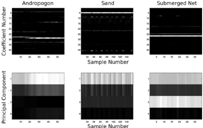
This method has recently seen a lot of attention in the fields of machine learn-ing, neuroscience and image processing[13, 24]. Just like PCA, sparse coding can serve as a dimensionality reduction tool. PCA tries to find a set of prin-ciple components that represents each pixel in the data, while sparse coding tries to train a dictionary whereby only a few elements will be used for the representation of a pixel[13]. This difference in data representation is illus-trated in figure 4. The goal of sparse representations is to find a set of vectors that serves the data while using a minimal number of nonzero elements. In order to find an optimal sparse code, the following minimization problem can be solved:

min

Z,D E(X,Z) =minZ,DkX−DZk 2

where X is the data, Dis the learned dictionary, Z is the sparse matrix and

αis a parameter controlling the influence of both terms. The partkX−DZk2₂

directly comes from the goal of the decomposition of signalXinDandZ(see equation (4.1)). Besides that decomposition, another goal is to use a minimal number of nonzero elements from the sparse matrixZ. Counting the number of nonzero elements ofZwill generally be done by usingkZk₀. Since this will make equation (4) a non-convex minimization problem and more sensitive for outliers, the `1-norm will be used instead[8]. The α in (4) determines how

much nonzero elements there are inZ. A largeαcauses thekZk₁to be small.

That means that Z can only contain a small number of nonzero elements. Whenαis small, the opposite result occurs.

There are cases where a fixed dictionary is suitable for finding a good sparse representation of the data, but in most cases learning a dictionary will drastic-ally improve the results of this method[6]. Although learned dictionaries im-prove the results, learning them is a computationally expensive procedure [22]. Fixed dictionaries typically lead to a fast transform but are limited in sparsifying the signals and can only be used for specific types of signals.

Figure 4: Three classes are represented by using a sparse representation and PCA as dimensionality reduction tool. The brighter the pixel, the higher the intensity of each coefficient. The three images in the second row show that PCA uses all the components to describe the classes, while the sparse repres-entation only uses several coefficients to describe the classes[13].

4.2

Dictionary learning

A dictionary based on training data can be learned in different ways. In this report an overcomplete (more columns than rows) dictionary is chosen because these dictionaries are more flexible and more resilient to noise[5]. Traditional learning methods for overcomplete dictionaries are based on it-erative batch methods, whereby in each iteration a cost function is minim-ized while addressing the training data. The most popular batch method is the K-means Singular Value Decomposition (K-SVD)[14, 28]. This method consists of two stages: calculation of a sparse matrix solving a version of equation 4 using a matching pursuit algorithm and a stage where the dic-tionary is updated column-by-column. Disadvantages of this method are its slow convergence[28] and the large memory requirement with large training data[24].

In [24] a method is introduced that solves these problems of K-SVD and is therefore used as the dictionary learning algorithm for this thesis. Below the two parts of the dictionary learning algorithm are listed. The result is a dic-tionary which is slightly overcomplete with 1000 columns (compared to the 943 spectral bands). A bigger dictionary was not an option due to computa-tional costs.

Algorithm 1Dictionary learning

1: functionDictionary learning(X,Z,D0,_α)

2: Require: x∈Rn _{∼ p(x)(random variable that randomly selects a} column),D0∈Rn×m_{,T(number of iterations)}

3: Initialize:A0=0,B0=0 4: fort=1 toTdo

5: Calculate sparse matrix using ISTA:

Zt=min Z

1

2kX−Dt−1Zk

2

2+αkZk1 (5)

6: At=At−1+ZtZtT 7: Bt=Bt−1+xtZtT

8: ComputerDtusing algorithm 2 withDt−1as input. 9: end for

10: Return DT (the learned dictionary) 11: end function

For the proof of convergence of algorithm 1 the following assumptions were needed[24]:

Assumption 1. The data meets a bounded probability density (i.e. the error in the data is bounded)

Assumption 2. The smallest eigenvalue ofAtis greater than or equal to a non-zero constant (i.e. Atinvertible).

Algorithm 2Dictionary update

1: functionDictionary update(D,A,B)

2: Require:D∈Rn×m_{dictionary from algorithm 1,} 3: A∈Rm×m_andB∈Rn×m

4: Repeat:

5: forj=1 tokdo

6: Update thej−th column ofD

uj = 1 Ajj

(bj−DAj) +Dj Dj = 1

max(u_j

2, 1) uj

(6)

7: end for

8: Until convergence

9: Return D(the updated dictionary)

4.3

Algorithms to compute sparse codes

The result of the presented method in paragraph 4.2 serves as input for the computation of the sparse matrix. Below two different algorithms are presen-ted that compute the algorithms. In the next paragraphs a short description is given and their pseudo codes.

4.3.1 ISTA

ISTA minimizes equation (4) overZ while fixing dictionaryD. The strength of this algorithm is its simplicity. The algorithm of ISTA is listed below[19]:

Algorithm 3ISTA

1: functionISTA(X,Z,D,α,L)

2: Require:L>largest eigenvalue ofDTD 3: Initialize:Z=0

4: repeat

5: Z=h_(α/L)(Z− 1_LDT(DZ−X)) 6: untilchange inZunder a threshold

whereby hα

L is the so-called shrinkage function. This shrinkage function can

be expressed as:

[hθ(V)]i=sign(Vi)(|V)i| −θi)+ (7) and is used to updateZiteratively with

Z[k+1] =h(α L)((I−

1

LD

T_D)Z[k]₊ 1

LD

T_{X). (8)}

This method has proven to converge, even with dense a data matrix[8].

4.3.2 CoD

Besides ISTA, the more efficient Coordinate Descent method (CoD) is intro-duced. Just like ISTA, a CoD method minimizes equation (4) overZwhile fix-ingD. The difference lies in the selection of components that will be changed per iteration. A CoD method selects one component to modify while ISTA modifies all components, causing a CoD method to converge faster. In al-gorithm 1Dhas the sizen×mand X n×k. That means that theZ is of the size m×k and therefore the computational complexity isO(mn), O(m2) or

O(ml)with l the average sparsity across samples and iterations. In CoD one component at a time is changed, which takesO(n)operations. This will be re-peated forO(n)orO(m)times and thus it is faster than ISTA. The algorithm of CoD is listed below[19]:

Algorithm 4Coordinate Descent

1: functionCoD(X,Z,D,_α,S) 2: Require:S=I−DTD 3: Initialize:Z=0,B=DTX 4: repeat

5: Z¯ =h_(α)(B)

6: k=index of largest component of|Z−Z|¯

7: ∀j∈[1,n]:Bj=Bj+Sjk(Z¯k−Zk) 8: Zk=Z¯k

9: untilchange inZunder a threshold

10: Z=hα(B) 11: end function

Since CoD updates only one component at a time, this algorithm is not per-forming a multivariate minimization but a scalar minimization subproblem instead. That means that every subproblem improves the estimation of the solution by minimizing along one direction while fixing others. This principle can easily be shown in 1D. The following minimization problem will then be solved[23]:

min

z∈RmE(z) =|z|1+λkDz−xk 2

2 (9)

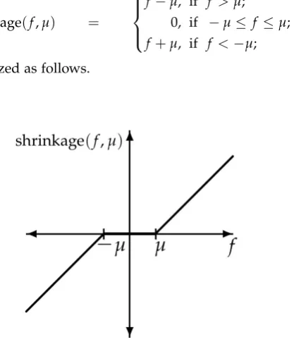
Minimizing this problem will deliver the same result as minimizing equation (4). The solution of this problem can be written as a shrinkage function where

shrinkage(f,µ) =   

 

f −µ, if f >µ;

0, if −µ≤ f ≤µ; f +µ, if f <−µ;

(10)

and can be visualized as follows.

5

Results

The method discussed in the last chapter is performed on a dataset containing 4 lymphocytes, 4 neutrophils, 4 breast cancer cells (SKBR3), 4 prostate cancer cells (PC3) and 4 LNCaP cells. PCA struggles with finding the distinction between LNCaP and SKBR3 and are therefore part of his dataset. Important is that only PCA is replaced and that the remainder of chapter 3 stays the same. The dictionary is learned in 25 iterations and based on this dictionary, ISTA and CoD are used for the calculation of the sparse matrix Z (see equation (4). This matrix is then used by HCA for making the clusters visible in a classification. Each simulation of ISTA is considered to be converted when

Z

[k+1]_−Z[k] ₂<1

and CoD is considered to be converted when 3500 iterations are reached or

Z

[k+1]_−Z[k] ₂<2.

Below results of minimizing equation (4) for different ISTA and COD, for different values ofαand 9 clusters are shown.

(a)Cancer cell classification withα=1.

(b)Cancer cell classification withα=200.

(c)Cancer cell classification withα=500.

Figure 6: Cancer cell classification for different values of α using ISTA. The

(a)Cancer cell classification withα=0.2.

(b)Cancer cell classification withα=50.

(c)Cancer cell classification withα=160.

Figure 7: Cancer cell classification for different values of α using CoD. The

cells used in this figure (from left to right): lymphocyte, breast cancer, prostate cancer and LNCaP.

Figure 6 shows that there is a value of α between 1 and 500 that describes

the data best. The value of α determines the extent to which the `1−norm

of the sparse matrix Zis dominant. For example, a high value of αensures

the `1−norm of Z to be small and consequently give a large value of θ in

equation (5). Because most components ofDandZare close to zero, thisθis

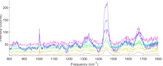
then a hard threshold and the shrinkage function[hθ(V)]i tends to go to zero for the utmost of the components. Therefore, as stated in figure 6c, a lot of pixels belong to the same red cluster at which it does not contribute anything to the classification. This is illustrated in figure 8 whereby it illustrates that the red cluster has a very low intensity. For the residual components the HCA tries to fit 9 clusters and is shown in the second (from left to right) illustration of figure 6c. Besides visual interpretation, unveiling the properties of the corresponding sparse matrix of α= 500, compared toα =200, gives a good

insight in the effect of a high value ofαfor the decomposition of signalY in DZ. Forα=500 the matrixZis nonzero for 0.54% of the elements and it uses

on average 5.44 elements to describe a pixel ofY(see equation (4.1)). That in comparison to 3.3% and 33.02 respectively forα=200.

Figure 7 also presents the fact that there is an optimal value for α for CoD.

Besides that, the difference in active components per pixel is also occurring for the CoD algorithm. In the case of α = 160 for CoD, only 0.45% of the

elements are nonzero and on average 4.53 elements are used to describe one pixel. On the other hand, 1.51% of the elements are nonzero forα =50 and

Figure 8:The measured intensity for the coloured clusters per frequency.

5.1

Optimizing

α

The figures above have shown that there is an optimal valueαfor this

classi-fication which describes the data best. For this optimization cluster validation tool Silhouette Validity Index (SVI) is used because this index can be used to test the input (Z) for the clustering for different values ofα and can also be

used for the determination of the number of clusters[7, 29]. SVI is an internal cluster validation index that is used in situations when no ground truth is known. Ground truth is data where the classification preferable has a high accuracy. The SVI for theith_{data point is defined as:}

Si=

bi−ai max(ai,bi))

, −1≤Si ≤1 (11)

where

(i) ai is the average Euclidean distance of the ith data point to all other points in the same cluster;

(ii) bi is the average Euclidean distance of the ith data point to all other points in the next nearest cluster.

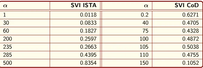
Below a table is shown with the SVIs from ISTA and CoD for different values ofα. For these calculations the number of clusters is kept constant at 9.

α SVI ISTA α SVI CoD

1 0.0118 0.2 0.6271

30 0.0833 40 0.4705

60 0.1827 75 0.4328

200 0.2597 100 0.4872

235 0.2663 105 0.5038

285 0.4395 110 0.4755

500 0.8354 150 0.1052

Table 1: Parameter optimization for ISTA and CoD using the SVI and 9 clusters.

The table shows that an increase inαensures an increase in SVI for the

out-puts of ISTA. The SVIs from CoD give a peak around the value α= 105 but

further analyis is needed to indicate the optimal value ofα. So based on this

validation tool alone an optimal value for αcan not be chosen and therefore

another internal validation index,Dunn’s validity index (DVI), is used for the determination of an optimal value of α. Just like the SVI, DVI also test the

input of this index (Z) and can be calculated as follows[7]:

D= min

1≤i≤k 

 min i+1≤j≤k





dist(ci,cj) max

1≤i≤kdiam(cl) 

 

 (12)

where

dist(ci,cj)is the distance between clusterci andcj. dist(ci,cj) =_x min

i∈ci,xj∈cj

d(xi,xj)

d(xi,xj)is the distance between data pointsxiandxj. diam(cl)is the diameter of clustercl where

diam(cl) =_xmax l,x2∈cl

d(x1,x2).

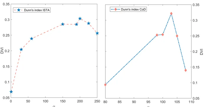
According to this tool, the higher the index the better the classification. Below in figure 9 the DVIs are calculated for several values ofα. Each calculated DVI

value is based on the average of 50 calculations because the DVI has not one specific value perαper iteration. The figure shows a clear peak atα=200 for

ISTA and atα=103 for CoD. Therefore, these values are used as the optimal

Figure 9:DVI for different values ofαusing ISTA and CoD.

5.2

Optimizing number of clusters

In the previous paragraph α = 200 is set as the optimal value for ISTA and α = 103 for CoD. These values are then used for the determination of the

optimal value for the number of clusters. Both SVI and DVI are used to determine this value and the results are shown in the table below.

# clusters SVI DVI

9 0.2597 0.3027

10 0.2594 0.2937

11 0.2594 0.2924

12 0.2602 0.3001

Table 2: Determination of the optimal number of clusters using the SVI and DVI on ISTA.

# clusters SVI DVI

9 0.4901 0.3216

10 0.4914 0.1864

11 0.4819 0.2685

12 0.4832 0.1334

Table 3: Determination of the optimal number of clusters using the SVI and DVI on CoD.

5.3

Comparison with PCA

For the comparison, the same validation tools are used for the classification of the method discussed in section 3. First, the classifications of the 5 different cancer cells are given below, then in table 4 the results of the validation tools are presented.

(a)SEM images from PC3 cell and the SKBR3.

(b)Difference in classification between CoD, ISTA and PCA (from top to down). From left to right: LNCaP, PC3, neutrophil, lymphocyte and SKBR3.

SVI DVI

ISTA 0.2597 0.3027

CoD 0.4901 0.3216

PCA 0.6166 0.0921

Table 4: Overview of the results of the validation tools SVI and DVI, using PCA and sparse coding.

5.4

Noise resilient

For testing the noise resilience of the algorithms PCA, ISTA and CoD, Gaus-sian noise is added to the data. Afterwards, the sparse matrix Zis calculated with the algorithms and the results are visually tested and validated with SVI and DVI. The corresponding probability density function is given as follows:

p(x) = 1

σ √

2π ·e−

(x−µ)2

2σ2

were µ and σ are the noise parameters. In this model the µ is set to 0 and σ to 1. Gaussian noise is a good method for testing the noise resilience of

algorithms because it resembles real world cases[12]. In table 5 the resulting SVI and DVI are presented and below the table the visual interpretation is shown.

SVI DVI

ISTA with noise 0.2534 0.2978

CoD with noise 0.4894 0.2705

PCA with noise 0.6103 0.0814

Table 5:Results of validation with ISTA using SVI and DVI.

Figure 12: Normal classification CoD (top) versus a classification with added Gaussian noise.

Figure 13: Normal classification PCA (top) versus a classification with added Gaussian noise.

5.5

Summary of the results

6

Conclusion & Recommendations

This report presented two methods based on sparse coding that were used to make hyperspectral camera data insightful. These dimensionality reduction algorithms, ISTA and CoD, made use of a pre-learned dictionary. The α of

equation (4) is optimized via two internal clustering validation tools. The proposed methods were applied to a data set containing 4 lymphocytes, 4 neutrophils, 4 breast cancer cells, 4 prostate cancer cells and 4 LNCaP cells.

Sparse coding has led to acceptable classifications of cancer cells and the cor-responding algorithms turned out to be resilient to noise. ISTA gave more clear distinctions between cancer cells than CoD. Based on the two internal validation tools it can not be said which algorithm, PCA or ISTA, is better at classifying cancer cells. This is because PCA had a higher SVI and ISTA scored better on the DVI. Besides that, both method were able to distinct neutrophils, lymphocytes and breast cancer, but were both not able to distinct LNCaP with PC3.

The results show that the resulting sparse model contains outliers and the model struggles to distinct the orange and red cluster (see the leftmost figure in figure 10b). If further research on this subject is conducted, I recommend to change a few parameters. In this research convergence for ISTA was reached

when

Z

[k+1]_−Z[k]

₂ < 1. Putting the norm difference closer to zero will

lead to a more converted solution of ISTA. This also applies for CoD, whereas there was not enough time to run the code longer. Besides that, the learned dictionary formed an input for ISTA and CoD and was learned within 25 iterations. In [13] was stated that most dictionaries were well-converted after 1000 iterations, but they recommend to upscale that number of iterations even more. Due to lack of a strong computer and time, I was not able to do these number of iterations. The 25 iteration and the large norm difference were therefore insufficient.

Besides this recommendation for longer computation time, I recommend to obtain the results based on more data. In this report 20 cancer cells in total are used for the input of the algorithms. More data and longer computations would improve the results of this research.

Besides more dictionaries, better understanding of the size of the dictionary would probably improve the classification. Expected is that there is an optimal size for this application but due to lack of time, this research has not been executed.

Furthermore, two internal classification validation tools are used for the op-timization ofαand the number of clusters. For a better optimization it would

References

[1] Cancer, key facts, howpublished = http://www.who.int/en/news-room/ fact-sheets/detail/cancer, note = Accessed: 2018-05-30.

[2] Pca notes. http://www.maths.manchester.ac.uk/~peterf/MATH38062/. Accessed: 2018-05-06.

[3] A. Castrodad, Z. Xing, J. G. E. B. L. C. and Sapiro, G. (2010). Discriminative sparse representations in hyperspectral imagery. Image Processing (ICIP), pages 1313–1316.

[4] Abdil, H. and Williams, L. J. (2010). Principal component analysis. WIREs Comp Stat, 2:433 – 459.

[5] Agarwal, A., Anandkumar, A., Jain, P., Netrapalli, P., and Tandon, R. (2014). Learning sparsely used overcomplete dictionaries. JMLR: Workshop and Conference Proceeding, pages 1–15.

[6] Aharon, M., Elad, M., and Bruckstein, A. (2006). K-svd: An algorithm for designing overcomplete dictionaries for sparse representation. IEEE TRANSACTIONS ON SIGNAL PROCESSING, 54:4311–4322.

[7] Ansari, Z., Azeem, M., Ahmed, W., and Babu, A. (2011). Quantitat-ive evaluation of performance and validity indices for clustering the web navigational sessions. World of Computer Science and Information Technology Journal(WCSIT), 1:217–226.

[8] Beck, A. and Teboulle, M. (2009). A fast iterative shrinkage-thresholding algorithm for linear inverse problems. SIAM J. Imaging sciences, 2:183–187.

[9] Behrmannl, J., Etmann, C., Boskamp, T., Casadonte, R., Kriegsmann, J., and Maass, P. (2018). Deep learning for tumor classification in imaging mass spectrometry. Bioinformatics, 34:1215–1223.

[10] Ben-Hur, A. and Guyon, I. (2003). Detecting stable clusters using prin-cipal component analysis. In Brownstein, M. and Kohodursky, A., editors,

Functional Genomics: Methods and Protocols, pages 159–182. Humana press.

[11] Bioucas-Dias, J. M., Chanussot, J., an Qian Du, N. D., Gader, P., Parente, M., and Plaza, A. (2012). Hyperspectral unmixing overview: geometrical, statistical, and sparse regression-based approaches. IEEE journal of slected topics in applied earth observations and remote sensing, 5:356–366.

[12] Boyat, A. K. and Joshi, B. K. (2015). A review paper: Noise models in digital image processing. Signal Image Processing : An International Journal (SIPIJ), 6:64–75.

[13] Charles, A. S., Olshausen, B. A., and Rozell, C. J. (2011). Learning sparse codes for hyperspectral imagery. IEEE journal of selected topics in signal pro-cessing, 5:963–965.

[15] Crowleya, E., Nicolantonio, F. D., Loupakis, F., and Bardelli, A. (2013). Liquid biopsy: monitoring cancer-genetics in the blood. Nature reviews, clinical oncology, 10:472–484.

[16] Cruz, M. R., Costa, R., and Cristofanilli, M. (2006). The

truth is in the blood: The evolution of liquid biopsies

in breast cancer management. https://am.asco.org/

truth-blood-evolution-liquid-biopsies-breast-cancer-management. Accessed: 2018-06-17.

[17] Enciso-Martinez, A., Timmermans, F. J., Nanou, A., Terstappen, L., and Otto, C. Sem-raman image cytometry of cells.The Royal Society of Chemistry.

[18] Field, D. J. and Olshausen, B. A. (1996). Emergence of simple-cell recept-ive field properties by learning a sparse code for natural images. Nature, 381:607–609.

[19] Gregor, K. and LeCun, Y. (2010). Learning fast approximations of sparse coding. Proceedings of the 27th international conference on machine learning.

[20] Holland, S. M. Principal components analysis (pca). https://strata. uga.edu/software/. Accessed: 2018-05-06.

[21] Ilie, M. and Hofman, P. (2016). Pros: Can tissue biopsy be replaced by liquid biopsy? Transl. Lung Cancer Res., 5:420–423.

[22] Julazadeh, M. (2012). Medical image segmentation and classification based on sparse representation and dictionary learning algorithms. Theses and dissertations, pages 13–17, 29–39.

[23] Li, Y. and Osher, S. (2009). Coordinate descent optimization for l1 minim-ization with application to compressed sensing; a greedy algorithm.Inverse Problems and Imaging, 3:487–503.

[24] Mairal, J. and Bach, F. (2009). Online dictionary learning for sparse cod-ing julien.International Conference on Machine Learning, 26.

[25] Neugebauer, U., Clement, J. H., Bocklitz, T., Krafft, C., and Popp, J. (2010). Identification and differentiation of single cells from peripheral blood by raman spectroscopic imaging.Journal of Biophotonics, 3:579–582.

[26] Rodarmel, C. and Shan, J. (2002). Principal component analysis for hyper-spectral image classification.Surveying and land information systems, 62:115– 118.

[27] Shalizi, C. Distances between clustering, hierarchical clustering. http: //www.stat.cmu.edu/~cshalizi/350/lectures/08/lecture-08.pdf. Ac-cessed: 2018-05-08.

[28] Tariyal, S., Majumdar, A., Singh, R., and Vatsa, M. Greedy deep diction-ary learning. CoRR, 54abs/1602.00203.

A

MATLAB implementations

A.1

The dictionary learning algorithm

function [X,beta]=dictionary(X,Y,Z,epsilon,alpha,L,theta,W) [a b]=size(X);

[c d]=size(Y);

A=zeros(b); B=zeros(a,b);

for t=1:50;

beta=ISTA(Y,Z,X,epsilon,alpha,L,theta,W);

A=A+beta*transpose(beta); %update A

B=B+Y*transpose(beta); %update B

X=dictionaryupdate(A,B,X); %upload dictionary

end end

A.2

The dictionary update

function [D_old]= dictionaryupdate(A,B,D) D_old=D;

[q,r]=size(D); D_new=zeros(q,r); norm_D=10;

eta=1; j=1;

while norm_D>eta;

for j=1:r;

if A(j,j)==0; %special treatment for singularities

u_j=(10^-14)*(B(:,j)-D_old*A(:,j))+D_old(:,j);

else

u_j=(1/A(j,j))*(B(:,j)-D_old*A(:,j))+D_old(:,j);

end

D_old(:,j)= (1/max(norm(u_j),1)).*u_j;

end

norm_D=norm(D_old-D_new) %check norm

D_new=D_old;

A.3

ISTA

function [W]=ISTArobust(input,Z,D,epsilon,alpha,L,theta) norm_ista=10;

W=Z-(1/L)*transpose(D)*(D*Z-input);

while norm_ista>epsilon; Z=W;

W=sign(Z-(1/L)*transpose(D)*(D*Z-input))

.*max(abs(Z-(1/L)*transpose(D)*(D*Z-input))-theta,0);

end end

A.4

CoD

function [Z]=CODrobust(X,Z,D,S,alpha,epsilon) B=transpose(D)*X;

norm_cod=10; Z_new=Z;

[a,b]=size(B); Z=zeros(a,b); k = 0;

while norm_cod(end)>epsilon && k < 3000 Z_bar=sign(B).*max(abs(B)-alpha,0); absolute=abs(Z-Z_bar);

[~, index] = max(absolute);

for i = 1:b

for j=1:a

B(j,i)=B(j,i)+S(j,index(i))

*Z_bar(index(i),i)-Z(index(i),i));

end

Z_new(index(i),i)=Z_bar(index(i),i);

end

norm_cod(end+1) = norm(Z_new-Z); Z=Z_new;

k = k + 1;

end

Z=sign(B).*max(abs(B)-alpha,0); plot(norm_cod)