Applications in Multivariate Signal Processing
Thomas Robert Diethe
A dissertation submitted in partial fulfillment of the requirements for the degree of
Doctor of Philosophy of the
University of London.
Department of Computer Science University College London
I, Thomas Robert Diethe, confirm that the work presented in this thesis is my own. Where informa-tion has been derived from other sources, I confirm that this has been indicated in the thesis.
Abstract
This thesis details theoretical and empirical work that draws from two main subject areas: Machine Learning (ML) and Digital Signal Processing (DSP). A unified general framework is given for the appli-cation of sparse machine learning methods to multivariate signal processing. In particular, methods that enforce sparsity will be employed for reasons of computational efficiency, regularisation, and compress-ibility. The methods presented can be seen as modular building blocks that can be applied to a variety of applications. Application specific prior knowledge can be used in various ways, resulting in a flexible and powerful set of tools. The motivation for the methods is to be able to learn and generalise from a set of multivariate signals.
In addition to testing on benchmark datasets, a series of empirical evaluations on real world datasets were carried out. These included: the classification of musical genre from polyphonic audio files; a study of how the sampling rate in a digital radar can be reduced through the use of Com-pressed Sensing (CS); analysis of human perception of different modulations of musical key from Electroencephalography (EEG) recordings; classification of genre of musical pieces to which a listener is attending from Magnetoencephalography (MEG) brain recordings. These applications demonstrate the efficacy of the framework and highlight interesting directions of future research.
Acknowledgements
To my parents, who have supported my education from start to finish, thank-you so much for giving me this opportunity. To my supervisor John Shawe-Taylor, whose breadth and depth of knowledge never ceases to amaze me, thank-you for your guidance.
The research leading to the results presented here has received funding from the EPSRC grant agreement EP-D063612-1, “Learning the Structure of Music”.
Contents
List of Figures 9
List of Tables 11
1 Introduction 12
1.1 Machine Learning . . . 12
1.2 Sparsity in Machine Learning . . . 12
1.3 Multivariate Signal Processing . . . 13
1.4 Application Areas . . . 14
1.4.1 Learning the Structure of Music . . . 14
1.4.2 Music Information Retrieval . . . 15
1.4.3 Automatic analysis of Brain Signals . . . 15
1.4.4 Additional Application Areas . . . 15
1.4.5 Published Works . . . 16
1.5 Structure of this thesis . . . 16
2 Background 18 2.1 Machine Learning . . . 18
2.1.1 Reproducing Kernel Hilbert Spaces . . . 19
2.1.2 Regression . . . 20
2.1.3 Loss functions for regression . . . 20
2.1.4 Linear regression in a feature space . . . 21
2.1.5 Stability of Regression . . . 22
2.1.6 Regularisation . . . 24
2.1.7 Sparse Regression . . . 25
2.1.8 Classification . . . 27
2.1.9 Loss functions for classification . . . 27
2.1.11 Boosting . . . 32
2.1.12 Subspace Methods . . . 37
2.1.13 Multi-view Learning . . . 38
2.2 Digital Signal Processing (DSP) . . . 39
2.2.1 Bases, Frames, Dictionaries and Transforms . . . 39
2.2.2 Sparse and Redundant Signals . . . 42
2.2.3 Greedy Methods for Sparse Estimation . . . 43
2.2.4 Compressed Sensing (CS) . . . 45
2.2.5 Incoherence With Random Measurements . . . 46
2.2.6 Multivariate Signal Processing . . . 47
3 Sparse Machine Learning Framework for Multivariate Signal Processing 48 3.1 Framework Outline . . . 48
3.2 Greedy methods for Machine Learning . . . 51
3.2.1 Matching Pursuit Kernel Fisher Discriminant Analysis . . . 51
3.2.2 Nystr¨om Low-Rank Approximations . . . 53
3.3 Kernel Polytope Faces Pursuit . . . 63
3.3.1 Generalisation error bound . . . 64
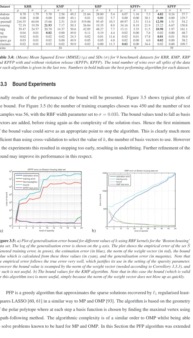
3.3.2 Experiments . . . 68
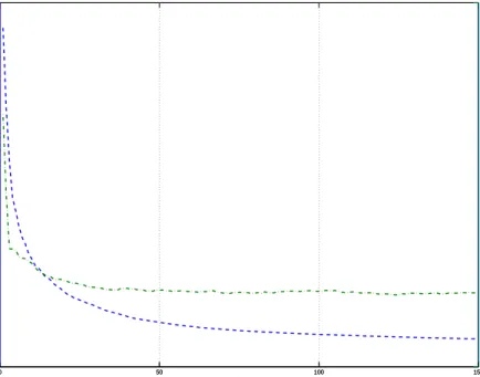
3.3.3 Bound Experiments . . . 69
3.4 Learning in a Nystr¨om Approximated Subspace . . . 70
3.4.1 Theory of Support Vector Machine (SVM) in Nystr¨om Subspace . . . 72
3.4.2 Experiments: Classification . . . 77
3.4.3 Experiments: Regression . . . 78
3.5 Multi-View Learning . . . 81
3.5.1 Kernel Canonical Correlation Analysis with Projected Nearest Neighbours . . . 83
3.5.2 Convex Multi-View Fisher Discriminant Analysis . . . 84
3.6 Conclusions and Further Work . . . 96
4 Applications I 97 4.1 Introduction . . . 97
4.2 Genre Classification . . . 98
4.2.1 MIREX . . . 99
4.2.2 Feature Selection . . . 100
4.2.3 Frame level features . . . 101
4.2.4 Feature Aggregation . . . 103
4.2.5 Algorithms . . . 103
4.2.6 Multiclass Linear Programming Boosting (LPBoost) Formulation (LPMBoost ) . 104 4.2.7 Experiments . . . 105
4.2.8 Results . . . 107
4.3 Compressed Sensing for Radar . . . 108
4.3.1 Review of Compressive Sampling . . . 109
4.3.2 Application of CS To Radar . . . 109
4.3.3 Experimental Approach . . . 110
4.3.4 Results And Analysis . . . 112
4.4 Conclusions . . . 117
5 Applications II 118 5.1 Introduction . . . 118
5.2 Experiment 1: Classification of tonality from EEG recordings . . . 119
5.2.1 Participants . . . 120 5.2.2 Design . . . 121 5.2.3 EEG Measurements . . . 121 5.2.4 Data Preprocessing . . . 121 5.2.5 Feature Extraction . . . 122 5.2.6 Results . . . 124 5.2.7 Leave-one-out Analysis . . . 126 5.3 Discussion . . . 127
5.4 Experiment 2: Classification of genre from MEG recordings . . . 128
5.4.1 Participants . . . 130 5.4.2 Design . . . 130 5.4.3 Procedure . . . 130 5.4.4 Feature Extraction . . . 131 5.4.5 Results . . . 132 5.4.6 Discussion . . . 134 6 Conclusions 135 6.1 Conclusions . . . 135 6.1.1 Greedy methods . . . 135
6.1.2 Low-rank approximation methods . . . 135
6.1.3 Multiview methods . . . 136
6.1.4 Experimental applications . . . 136
6.2 Further Work . . . 139
6.2.1 Synthesis of greedy/Nystr¨om methods and Multi-View Learning (MVL) methods 139 6.2.2 Nonlinear Dynamics of Chaotic and Stochastic Systems . . . 140
6.3 One-class Fisher Discriminant Analysis . . . 141
6.4 Summary and Conclusions . . . 142
B Acronyms 144
List of Figures
2.1 Modularity of kernel methods . . . 19
2.2 Structural Risk Minimisation . . . 24
2.3 Minimisation onto norm balls . . . 26
2.4 Some examples of convex loss functions used in classification . . . 28
2.5 Common tasks in Digital Signal Processing . . . 39
3.1 Diagrammatic view of the process of machine learning from multivariate signals . . . 50
3.2 Diagrammatic representation of the Nystr¨om method . . . 54
3.3 Plot of generalisation error bound for different values ofkusing RBF kernels . . . 62
3.4 Plot showing how the norm of the deflated kernel matrix and the test error vary withk. . 63
3.5 Generalisation error bound for the ‘Boston housing’ data set . . . 69
3.6 Plot of f(ǫ) = (1−ǫ/2) ln(1 + 1ǫ/−2ǫ)−ǫ/2 and f(ǫ) =8 ǫ for ǫ∈ {0,0.5} . . . 76
3.7 Error and run-time as a function ofkon ‘Breast Cancer’ for NFDA, KFDA . . . 79
3.8 Error and run-time as a function ofkon ‘Flare Solar’ for NFDA, KFDA . . . 80
3.9 Error and run-time as a function ofkon ‘Bodyfat’ by KRR, NRR and KRR . . . 81
3.10 Error and run-time as a function ofkfor ‘Housing’ by KRR, NRR and KRR . . . 82
3.11 Diagrammatic view of the process of a) MSL, b) MVL and c) MKL . . . 83
3.12 Plates diagram showing the hierarchical Bayesian interpretation of MFDA . . . 87
3.13 Weights given by MFDA and SMFDA on the toy dataset . . . 94
3.14 Average precision recall curves for 3 VOC 2007 datasets for SMFDA and PicSOM . . . 95
4.1 Confusion Matrix of human performance on Anders Meng dataset d004 . . . 106
4.2 The modified receiver chain for CS radar. . . 109
4.3 Fast-time samples of the stationary target. . . 112
4.4 Range profiles of the stationary target. . . 113
4.5 Fast-time samples constructed from largest three coefficients. . . 113
4.6 Range profiles constructed from largest three coefficients. . . 114
4.8 Range-frequency surfaces for van target using CS. . . 114
4.9 Range-frequency surfaces for person target using CS. . . 115
4.10 DTW applied to the person target . . . 116
4.11 DTW applied to the van target . . . 117
List of Tables
2.1 Common loss functions and corresponding density models . . . 21
2.2 Example of the dyadic sampling scheme . . . 42
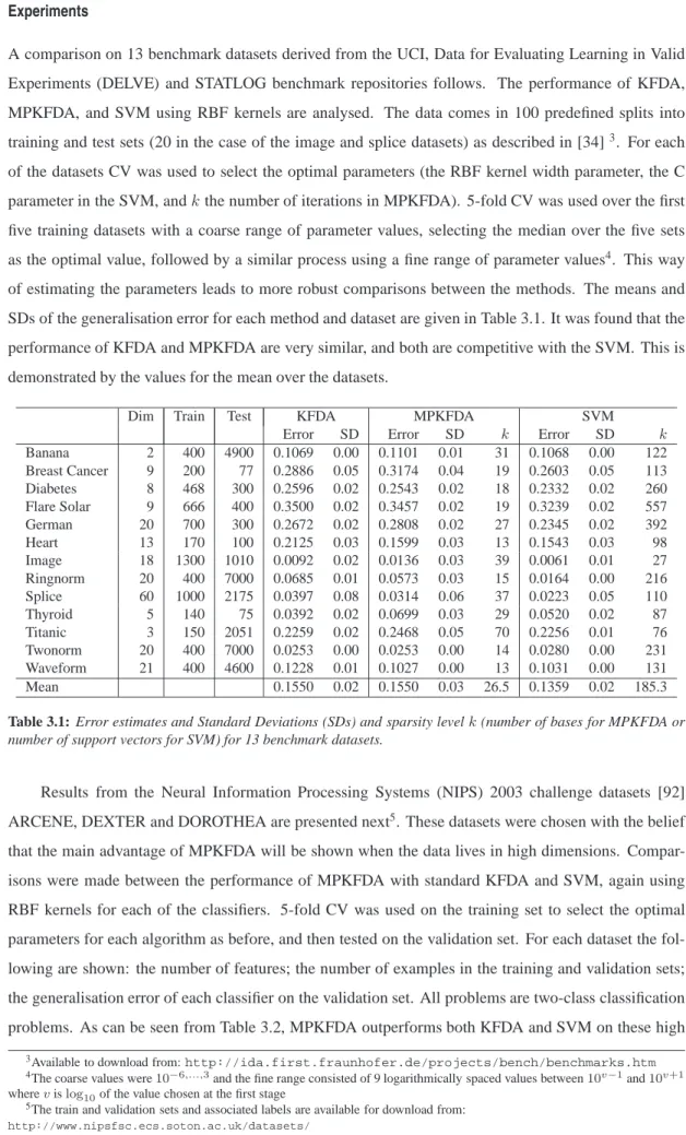
3.1 Error estimates and Standard Deviations (SDs) for MPKFDA on 13 benchmark datasets . 60 3.2 Error estimates for MPKFDA on 3 high dimensional datasets. . . 61
3.3 Number of examples and dimensions of each of the 9 benchmark datasets . . . 68
3.4 MMSE and SDs for 9 benchmark datasets for KRR, KMP, KBP and KPFP . . . 69
3.5 Error estimates and SDs for 13 benchmark datasets for SVM, NSVM . . . 78
3.6 Error estimates and SDs for 13 benchmark datasets for KFDA, NFDA, and MPKFDA . . 78
3.7 MMSE and SDs for 7 benchmark datasets for KRR, NRR, and KMP . . . 79
3.8 Test errors over ten runs on the toy dataset . . . 93
3.9 BER and AP for four VOC datasets, for PicSOM, KFDA CV,ksumand MFDA . . . 94
3.10 Leave-one-out errors for each subject for SVM, KCCA/SVM, and MFDA . . . 96
4.1 Summary of results of the Audio Genre Classification task from MIREX 2005 . . . 100
4.2 An example of the augmented hypothesis matrix . . . 105
4.3 Classification accuracy on ‘Magnatune 2004’ for AdaBoost, LPBoost and LPMBoost . . 107
4.4 Classification accuracy on ‘MENG(4)’ for AdaBoost, LPBoost, and LPMBoost . . . 107
4.5 The normalized errors for the moving targets . . . 115
4.6 Effect of Dynamic Time Warping (DTW) . . . 116
5.1 Test errors for within-subject SVM classification . . . 124
5.2 Test errors for leave-one-out SVM classification using linear kernels . . . 125
5.3 Test errors for within-subject classification using KCCA/PNN and SVM classification . . 126
5.4 Test errors for leave-one-subject-out KCCA/PNN . . . 127
5.5 MIDI features used for genre classification . . . 131
5.6 Confusion matrix for classification of genre by participants . . . 132
Chapter
1
Introduction
1.1
Machine Learning
ML is a relatively young field that can be considered an extension of traditional statistics, with influences from optimisation, artificial intelligence, and theoretical computer science (to name but a few). One of the fundamental tenets of ML is statistical inference and decision making, with a focus on prediction performance of inferred models and exploratory data analysis. In contrast to traditional statistics, there is less focus on issues such as coverage (i.e. the interval for which it can be stated with a given level of confidence contains at least a specified proportion of the sample). In statistics, classical methods rely heavily on assumptions which are often not met in practice. In particular, it is often assumed that the data residuals are normally distributed, at least approximately, or that the central limit theorem can be relied on to produce normally distributed estimates. Unfortunately, when there are outliers in the data, classical (linear) methods often have very poor performance. This calls for theoretically justified non-linear methods which require fewer assumptions. This is the approach that will be taken throughout this thesis, with a focus on developing a computational methodology for efficient inference with empirical evaluation. This will be backed up through analysis drawn from statistical learning theory, which allows us to make guarantees about the generalisation performance (or other relevant properties) of particular algorithms given certain assumptions on the classes of data.
1.2
Sparsity in Machine Learning
In information theory, the concept of redundancy is defined as the total number of bits used to transfer a message minus the number of bits of actual information in the signal. In ML redundancy appears in data in many forms. Perhaps the most common is noise - whether this is measurement noise or system noise - but there are also often domain specific sources of redundancy due to the nature of the data itself (i.e. high self-similarity) or to the way in which it is collected. In the particular application domains of interest in this thesis, namely multivariate signals, we are faced with potentially high levels
of both of these type of redundancy. Whenever there is redundancy in a dataset, there is the potential for sparse representations. In its most literal form, sparsity may involve a reduction in the number of data dimensions (“dimensionality reduction”), or in the number of examples needed to represent a pattern (“sample compression”). These two types of sparsity are known as “primal” and “dual” sparsity respectively, due to the concept of duality from the optimisation community (see e.g. [1]). Both of these types of sparsity have attractive properties, including:
• data compression,
• subset or feature selection,
• statistical stability (in terms of the generalisation of patterns),
• robustness (i.e. to outliers or small departures from model assumptions), • space efficiency, and
• faster computations (after learning).
One of the biggest drawbacks of sparse methods tends to be in terms of computational efficiency during learning. Much of the work in this thesis will be focussed on optimisation methods for sparse learning that are computationally efficient. The most well known examples of sparse methods in statistics and ML include methods such as the Least Absolute Shrinkage and Selection Operator (LASSO) [2] and SVM [3], which are sparse in the primal and dual respectively. There are close relations between both of these methods as outlined by [4], and indeed with many other sparse methods such as LPBoost [5] and Kernel Basis Pursuit (KBP) [6]. Other classes of sparse methods include greedy methods such as Kernel Matching Pursuit (KMP) and methods based on random subsampling such as the Nystr¨om method [7]. Chapter 2 will outline these and other methods and try to emphasise the linkage between them, whilst Chapter 3 builds on these methods to produce novel algorithms that are theoretically motivated and empirically validated.
1.3
Multivariate Signal Processing
As already alluded to, the specific class of data that will be the particular focus of this thesis is multi-variate signals. The issues of redundancy and sparsity are particularly magnified within this domain, as the sensors used to gather the signals are often spatially proximal, and as a result their measurements are often highly correlated. In addition, many real-world signals are affected by a high degree of noise (which can be systemic noise or measurement noise). Finally, due to high rates of sampling and dense sensor grids, the data is often extremely high dimensional. It is therefore especially important that the methods used are capable of learning in this difficult domain.
Standard batch or online ML methods often fall short when analysing signals because the data violates one of the basic assumptions: that the data is independently and identically distributed (i.i.d.). There are of course a range of ML methods that deal specifically with non-i.i.d. data and in particular time series data, but the models are often highly complex and do not scale well to large datasets. In particular, these approaches often become intractable in the multivariate case - when we are dealing with
large sets of signals (as is often the case in biological applications, for example). Another approach to take is to break the signal into “chunks”, perform a series of DSP operations on these chunks, and use the resulting data as examples in standard ML algorithms. Whilst the i.i.d. assumption is still violated, its impact is often softened as significant integration over time takes place. However care must be taken to avoid learning trivial relations due to this issue. The major benefit of this approach is that it means the problem of inference on signals can be “modularised”, i.e. broken into subproblems, and subsequently highly developed methods from both DSP and ML can be applied. This approach will form the basis of the machine learning framework for multivariate signal processing that will be outlined in Chapter 3.
The links between DSP and ML run very deep, often with the same mathematical methods being used for different applications. In essence, both fields are interested in the solutions to underdetermined problems, inverse problems, and sparse estimation (see e.g. [8]). This means that there is fertile ground for cross-pollination of ideas; for example in Section 3.2 I will show how “greedy” methods from DSP can be used to solve ML optimisation problems, and use statistical learning theory analysis to give guarantees on the performance of the resulting algorithms.
1.4
Application Areas
1.4.1
Learning the Structure of Music
The funding and therefore main application area for this thesis was the EPSRC project entitled “Learning the Structure of Music”, which encompasses three fields of science, music cognition, representation, and machine learning. The project was a collaborative effort between the Centre for Computational Statis-tics and Machine Learning at University College London, the Interdisciplinary Centre for Computer Music Research at the University of Plymouth, the Leibniz Institute for Neurobiology at the Univer-sity of Magdeburg, and the Department of Computational Perception at the Johannes Kepler UniverUniver-sity Linz. The aims of the project were to develop models and tools that apply novel signal processing and machine learning techniques to the analysis of both musical data and brain imaging data on music cog-nition. The metrics of success for the project were in terms of both theoretical results and experimental results. Specifically, the goals were to deepen the understanding of the relationship between musical structure and musical performance, quantifiable by the ability to predict performer styles; to deepen the understanding of the relationship between musical structure and listening experience, quantifiable by the ability to predict patterns of brain activity; and to develop systems for generative performance and music composition, quantifiable by the ability to generate coherent musical performances and compositions.
The experimental research that falls within the scope of this thesis seeks to find common patterns be-tween the features extracted from polyphonic music, and the representation of musical structures within the brain through the use of EEG and MEG recordings. This thesis is therefore targeted at the first two of the three goals described above. To this end, the experimental research initially naturally followed two paths, namely the understanding of polyphonic audio signal and of brain activity recordings, before integrating the two to search for common patterns. Each of these stages will be described in detail.
1.4.2
Music Information Retrieval
In the first part of the research, the goal was to investigate techniques for extracting features from mu-sic in two forms: score-based representations (e.g. Mumu-sical Instrument Digital Interface (MIDI)), and polyphonic music (e.g. Waveform Audio File Format (WAVE) audio). As most musical pieces are not available in the former of these representations, and the signal processing required to extract information from polyphonic audio is much more complicated, the research focussed on polyphonic audio. When available, however, score-based representations provide a rich source of information and this led to their use in later experiments involving human subjects. A broad range of audio features were considered, including musical structure, melody, harmony, chord sequences, or more general spectral or timbral characteristics. An initial survey of the field identified that classification of musical genre from audio files, as a fairly well researched area of music research, provided a good starting point. What would appear on the surface to be a relatively trivial task, is in reality difficult for a number of reasons, not least that the concept of a genre is rather subjective and amorphous. However despite these shortcomings, useful progress has been made in this area, including insights into the types of features that are appro-priate for this kind of task and the types of algorithm best suited to the classification problem. Chapter 4 describes research into this area, and includes a description of the novel approach taken, as well as a discussion of the complications unearthed by this research.
1.4.3
Automatic analysis of Brain Signals
Neuroscience, like many other areas of science, is experiencing a data explosion, driven both by improve-ments in existing recording technologies, such as EEG, MEG, Positron Emission Tomography (PET), and functional Magnetic Resonance Imaging (fMRI). The improvements increase the quantity of data through these technologies have had a significant impact on basic and clinical neuroscience research. An analysis bottleneck is inevitable as the collection of data using these techniques now outpaces the development of new methods appropriate for analysis of the data, and the dimensionality of the data increases as the sensors improve in spatial and temporal resolution.
1.4.4
Additional Application Areas
Traditional processing of digital radar relies on sampling at the Nyquist frequency - i.e. twice the fre-quency of the highest part of the bandwidth required. This requires extremely fast and expensive Ana-logue to Digital Conversion (ADC) equipment, often operating at rates of up to 1GHz. Methods that can reduce the frequency at which the ADC operates, or alternatively increase the signal bandwidth whilst operating at the same frequency, would be of great benefit to the radar community. A form of Compressed Sensing (CS) known Analogue to Information Conversion (AIC) [9, 10] that reduces the sampling frequency from the traditional Nyquist rate by sampling at the information rate, rather than the rate required to accurately reproduce the baseband signal, will be applied to real radar data in 4.
1.4.5
Published Works
The following publications have resulted from this work, and will be referenced where appropriate in the text.
Peer reviewed technical reports
Diethe, T., & Shawe-Taylor, J. (2007). Linear Programming Boosting for the Classification of Mu-sical Genre. Technical Report Presented at the NIPS 2007 workshop Music, Brain & Cognition. [11]
Diethe, T., Durrant, S., Shawe-Taylor, J., & Neubauer, H. (2008). Semantic Dimensionality Re-duction for the Classification of EEG according to Musical Tonality. Technical Report Presented at the NIPS 2008 workshop Learning from Multiple Sources. [12]
Diethe, T., Hardoon, D.R., & Shawe-Taylor, J. (2008). Multiview Fisher Discriminant Analysis. Technical Report Presented at the NIPS 2008 workshop Learning from Multiple Sources. [13]
Peer reviewed conference papers
Diethe, T., Durrant, S., Shawe-Taylor, J., & Neubauer, H. (2009). Detection of Changes in Patterns of Brain Activity According to Musical Tonality. Proceedings of IASTED Artificial Intelligence and Applications. [14]
Diethe, T., Hussain, Z., Hardoon, D.R., & Shawe-Taylor, J. (2009). Matching Pursuit Kernel Fisher Discriminant Analysis. Proceedings of the 12th International Conference on Artificial In-telligence and Statistics (AISTATS) 2009, 5, 121-128. [15]
Diethe, T., Teodoru, G., Furl, N., & Shawe-Taylor, J. (2009). Sparse Multiview Methods for Classification of Musical Genre from Magnetoencephalography Recordings. Proceedings of the 7th Triennial Conference of European Society for the Cognitive Sciences of Music (ESCOM 2009) Jyvskyl, Finland, online athttp://urn.fi/URN:NBN:fi:jyu-2009411242. [16] Diethe, T., & Hussain, Z. (2009). Kernel Polytope Faces Pursuit. Proceedings of ECML PKDD 2009, Part I, LNAI 5781, 290-301. [17]
Smith, G.E., Diethe, T., Hussain, Z., Shawe-Taylor, J., & Hardoon, D.R. (2010). Compressed Sampling For Pulse Doppler Radar. Proceedings of RADAR 2010. [18]
1.5
Structure of this thesis
The work in this thesis draws from several disparate areas of research, including digital signal processing, machine learning, statistical learning theory, psychology, and neuroscience. The next Chapter (2) will introduce some concepts from signal processing and machine learning that underly the theoretical and algorithmic developments, which are linked together into a coherent framework in Chapter 3. The fol-lowing two Chapters, 4 and 5, will describe the experimental work described above in more detail, with
a focus on univariate and multivariate signal processing respectively. The final Chapter (6) concludes by giving some philosophical insights and discussion of intended future directions.
Chapter
2
Background
Abstract
Space and Time. In this chapter I will provide background information for the two main subject areas that form the basis of the thesis: Machine Learning and Signal Processing. Machine Learning is a field that has grown from other fields such as Artificial Intelligence, Statistics, Pattern Recognition, Optimisation, and Theoretical Computer Science. The core goal of the field is to find methods that learn statistical patterns within data that are generalisable to unseen data using methods that are efficient and mathematically grounded. Signal processing is broader in the sense that there are multiple goals, such as control, data compression, data transmission, denoising, filtering, smoothing, reconstruction, identification etc., but narrower in the sense that it (generally) focusses on time-series data (which can be continuous or discrete, real or complex, univariate or multivariate). Where these fields intersect interesting challenges can be found that drive development in both fields.
2.1
Machine Learning
An important feature of most developments in the field of ML that is derived directly from a computer science background is the notion of modularity in algorithm design. Modular programming (also known as ‘Divide-and-Conquer’) is a general approach to algorithm design which has several obvious advan-tages: when a problem is divided into sub-problems, different teams/programmers/research groups can work in parallel, reducing programme development time; programming, debugging, testing and mainte-nance are facilitated; the size of modules can be reduced to a humanly comprehensible and manageable level; individual modules can be modified to run on other platforms; modules can be re-used within a programme and across programmes. In the context of ML, modularity exists due to the existence of so called kernel functions (which will be explained below), which allow the problem of learning to be decomposed into the following stages: preprocessing, feature extraction, kernel creation (or alter-natively weak-learner generation - see Section 2.1.11), and learning. This flow is depicted in Figure
2.1. Common to both ML and DSP is a desire not only to find solutions to problems, but also to do so Pre-processing Feature extraction K(xi,xj) Kernel Function αi Learning algorithm Output f(xi) xi Data Subspace Projection
Figure 2.1: Modularity of kernel methods
efficiently. Drawing from optimisation theory, much work revolves around trying to find more efficient methods for solving problems that are exactly correct or approximately correct. The choice of optimi-sation method often comes down to a trade-off between computation time and memory requirements, or alternatively between accuracy of solutions and the time it takes to achieve them. Much of the focus of the next Chapter will be on different optimisation methods to achieve sparse solutions in computa-tionally efficient ways. These methods include convex optimisation, iterative “greedy” methods, and methods that involve random subsampling or random projections. Examples of each of these methods will be introduced later in this Chapter.
ML deals with a wide variety of problems, from ranking of web-pages to learning of trading rules in financial markets. However the present focus will be on the more fundamental problems of classifica-tion, regression (function fitting and extrapolation), subspace learning and outlier detection. Many more complex tasks can be decomposed into these fundamental tasks, so it is important to focus on the foun-dations before building up to more complex scenarios. However common to all of the tasks is a focus on the generalisation ability of learnt models, so this will be the key metric upon which the empirical validation is grounded.
The first part of the Chapter will introduce some of the basic concepts mentioned above, firstly ML methods: regression, classification, regularisation, margin maximisation, boosting, subspace learning, and MVL; following from this will be DSP concepts such as dictionaries, bases, sparse representations, multivariate signal processing, and compressed sensing. Theoretical insights from Statistical Learning Theory (SLT) will be used to justify the methods as they are introduced.
2.1.1
Reproducing Kernel Hilbert Spaces
Outside of ML, the Reproducing Kernel Hilbert Spaces (RKHS) method provides a rigorous and ef-fective framework for smooth multivariate interpolation of arbitrarily scattered data and for accurate approximation of general multidimensional functions. Given a Hilbert spaceHand an examplexi, the
reproducing property can be stated as follows,
f(xi) =hf, κ(xi,·)iH (2.1)
of the reproducing kernelκfor every functionf(xi)belonging toH. This property allows us to work in
the implicit feature space defined only with the inner products, and is the key to kernel methods for ML. This allows inner products between nonlinear mappingsφ:xi →φ(xi)∈ Fofxiinto a feature
cases, this inner product or kernel function (denoted byκ) can be evaluated much more efficiently than the feature vector itself, which can even be infinite dimensional in principle. A commonly used kernel function for which this is the case is the Radial Basis Function (RBF) kernel, which is defined as:
κRBF(xi,xj) = exp −kxi−xjk 2 2σ2 . (2.2)
2.1.2
Regression
Given a sampleScontaining examplesx∈Rnand labelsy ∈R. LetX= (x1, . . . ,xm)′be the input
vectors stored in matrixXas row vectors, where′denote the transpose of vectors or matrices.
Table A.1 in Appendix A is included as reference for some of the more commonly used mathemat-ical symbols.
The following assumptions will be made in order to aid presentation: Data is centered (or alterna-tively a column of ones can be added as an extra feature, which will function as the intercept); the data is generated i.i.d. according to an unknown but fixed distributionD. Furthermore, a Gaussian noise model with zero mean is assumed.
2.1.3
Loss functions for regression
Before going on to give specific examples of learning algorithms for regression, it is worth introducing the different loss functions that are commonly used for regression, along with their relation to the noise model.
Defining the square loss as
L{2}=kf(x)−yk22, (2.3)
whereyˆ=f(x)is the estimate of the outputsy. This is also known as Gaussian loss as minimising this loss is the Maximum Likelihood solution if a Gaussian noise model is assumed. Alternatively we can denote the vector of slack variablesξ=|y−yˆ|as the differences between the true and estimated labels, and we divide by a half to make algebra easier, giving
L{2}=
1 2kξk
2
2. (2.4)
Theℓ1loss is similarly defined as,
L{1} =kξk1, (2.5)
Loss functionalL(ξ) density modelp(ξ) ǫ-insensitive kξkǫ 2(1+1ǫ)exp (− kξkǫ) Laplacian kξk1 12exp (− kξk1) Gaussian 12kξk22 √1 2πexp −kξk22 2
Huber’s robust loss 1 2σkξk 2 2 if|ξ| ≤σ |ξ| −σ2 otherwise ∝ ( exp−ξ2 2σ if|ξ| ≤σ exp σ 2 − |ξ| otherwise Polynomial 1d|ξ|d 2Γ(1d/d)exp− |ξ|d
Table 2.1: Common loss functions and corresponding density models, adapted from [19]
a region of widthǫaround zero within which deviations are not penalised leads to theǫ-insensitive loss, L{ǫ,1}= max (kξk1−ǫ,0)
.
=kξkǫ,1, for theℓ1noise model, and (2.6)
L{ǫ,2}= max (kξk2−ǫ,0)
.
=kξkǫ,2, for theℓ2noise model. (2.7)
Some loss functions and their equivalent noise models are given in Table 2.1. For simplicity, the rest of this Section will use the square loss of Equation 2.3. However any of the loss functions given (or other loss functions not given due to space constraints) can be substituted to give different optimisation criteria. This approach is known as the General Linear Model (GLM). In all of the cases outlined here, the loss function is convex which leads to exact optimisation problems. However, non-differentiable loss functions such as the linear loss or theǫ-insensitive loss are typically harder to solve.
2.1.4
Linear regression in a feature space
Assume that data is generated according to a linear regression model,
yi=xiw+ni, (2.8)
wherenis assumed to be an i.i.d. random variable (noise) with mean0and variance σ2. LetX = (x1, . . . ,xm)′ be the input vectors stored in matrixX as row vectors, andy = (y1, . . . ,ym)′ be a
vector of outputs. Assume the square loss as defined in Equation 2.3, as this is the Maximum Likelihood solution to the linear regression problem of Equation 2.8. Intuitively it makes sense as the squaring of the errors places emphasis on larger errors whilst ignoring the sign. The formulation for linear regression that minimises this loss is then given by,
min w L(X,y,w) (2.9) = min w kXw−yk 2 2. (2.10)
By differentiating with respect tow, equating to zero and rearranging, it can be seen that there is a closed form solution forw∗,
w∗ = (X′X)−1X′y, (2.11)
provided that the matrixX′Xis invertible. The dual of this optimisation is formed as follows,
min α kXX ′α−yk2 2 (2.12) = min α kKα−yk 2 2, (2.13)
which in turn has a closed form solution,
α∗= (XX′)−1y, (2.14)
=K−1y, (2.15)
again provided that the matrixXX′is invertible. The function to test this model on a new data point is given by,
f(xi) =K(i,·)α∗. (2.16)
This kernel trick is based on the reproducing property introduced in Section 2.1.1, with the observation that in the equation to computeα∗(2.24) as well as in the equation to evaluate the regression function (2.16), all that is needed are the vectorsxiin inner products with each other. It is therefore sufficient to
know these inner products only, instead of the actual vectorsxi. Observe that the kernel regression form
of Equation 2.15 when used with an RBF kernel has higher capacity than the linear regression form of Equation 2.11, i.e. it allows for a richer class of functions to be learnt than by the standard linear model. Whilst this increase in capacity may be desirable if the data is not in fact linear, in the presence of noise this can cause problems due to the ability of the model to fit the noise (overfitting). In this situation, some form of capacity control is required.
2.1.5
Stability of Regression
In statistics, this capacity control can be seen through what is known as the bias variance trade-off [20]. Typically, a model with low capacity such as the linear model of Equation 2.11, will have high bias as it will fit only a very restricted class of data, whilst the variance is low as perturbing some of the data points will have little effect. In contrast, if a high capacity model is used such as Equation 2.15 with the RBF kernel as defined in (2.2), the function can fit the data exactly (low bias) but if even a single data point is perturbed the function will change drastically (high variance). Hence it would be desirable to optimise the trade-off between these two in order to generate models with predictive power on new data. This is closely related to the concepts of overfitting and regularisation that will be discussed in Section
2.1.6.
McDiarmid’s inequality [21], which is a generalization of Hoeffding’s inequality [22], is a result in probability theory that gives an upper bound on the probability for the value of a function depending on multiple independent random variables to deviate from its expected value. This is a result that comes from the law of large numbers by Chernoff in relation to the convergence of Bernoulli trials [23]. The risk associated with a functionf is defined as the expectation of the loss function,
R=Ex,y∈{X ×Y}[L(f(x, y))], (2.17) and the empirical risk as the expectation of a particular sampleS,
ˆ R=Ex,y∈S[L(f(x)] = 1 m m X i=1 L(f(xi, yi)). (2.18)
Given random variablesxilying in the range[ai, bi], the probability that the expected empirical riskRˆ
differs from the true risk (or error)Rby a valueǫcan be bounded as follows,
Pr|R − R| ≥ˆ ǫ≤2 exp − 2mǫ 2 (b−a)2 , (2.19)
This shows that there is an exponential decay of the difference in the probabilities as the sample size increases. This gives us a clue that to learn well, the best thing that one can do is to increase the amount of data available. However, if this is not possible, the only other option is to control the capacity of the the learning algorithm.
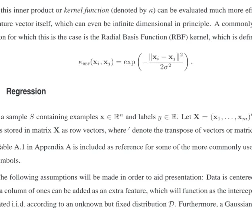
Another viewpoint introduced by Vapnik and Chervonenkis is the notion of Structural Risk Minimisation (SRM) [24, 25, 26]. The real errorRis upper bounded by the empirical errorRˆ and another value called the structural riskRS. The structural risk is a theoretical criterion that can be
com-puted for certain classes of models and estimated in most other cases. Choose the model that achieves the lowest upper bound.
R= ˆR+RS. (2.20)
The idea is to impose a structure on the class of admissible functionsF, such that each individual functionfj which has lower capacity than the nextfj+1. This is depicted diagrammatically in Figure
2.2. Another closely related approach to capacity control is regularisation, which will be discussed below in Section 2.1.6. If we choose to control the capacity using a class of functions with bounded norm, we are in fact using the set of regularised functions, which gives an additional justification for this type of regularisation.
VC-Dimension (
h
)
Error
Bound on true error
Capacity
Empirical error
R
(
f
∗)
f
j−1⊂
f
j⊂
f
j+1. . .
⊂
⊂
. . .
Figure 2.2: Structural Risk Minimisation (adapted from [19]). The principle is to find the optimal functionf∗ that satisfies the trade-off between low capacity and low training error
2.1.6
Regularisation
Inverse problems, such as (2.22) and (2.24) are often ill-posed. This is usually due to the condition number1of the matrix to be inverted, meaning that it needs to be re-formulated for numerical treatment.
Typically this involves including additional assumptions, such as smoothness of solutions. This process is known in the statistics community as regularisation, and Tikhonov regularisation is one of the most commonly used types of regularisation for the solution of linear ill-posed problems [27]. There is also a secondary reason why regularisation is important: overfitting. Overfitting occurs when an inferred model describes the noise in the data rather than the underlying pattern. Overfitting generally occurs when the complexity of the model is too high in relation to the quantity of data available (i.e. in terms of degrees of freedom). A model which has been overfit will generally have poor generalisation performance on unseen data. Tikhonov regularisation is defined as,
min w kXw−yk 2 2+kΛwk 2 2, (2.21)
whereΛ is the Tikhonov matrix. Although at first sight the choice of the solution to this regularised problem may look artificial, the process can be justified from a Bayesian point of view. Note that for an ill-posed problem one must necessarily introduce some additional assumptions in order to get a stable solution. A statistical assumption might be that a-priori it is known thatXis a random variable drawn from a multivariate normal distribution, which for simplicity is assumed to be mean zero and that each component is independent with standard deviationσx. The data is also subject to noise, and we take the
errors inyto be also independent with zero mean and standard deviationσy. Under these assumptions,
according to Bayes’ theorem the Tikhonov-regularized solution is the most probable solution given the data and the a-priori distribution of X. The Tikhonov matrix is then Λ = λI for Tikhonov factor λ = σy/σx. Of course this Tikhonov factor is not known, so must be estimated in some way. If the
assumption of normality is replaced by assumptions of homoscedasticity and that errors are uncorrelated, and still assume zero mean, then the Gauss-Markov theorem implies that the solution is a minimal unbiased estimate [28].
It is therefore justified to set the Tikhonov matrix to be a multiple of the identity matrixΛ = λI; this method is known in the statistics and ML literature as Ridge Regression (RR).
Ridge Regression
The primal formulation for RR is therefore given by,
min w kXw−yk 2 2+λkwk 2 2. (2.22)
Similarly to (2.11), a closed form solution for RR exists,
w∗= (X′X+λI)−1X′y. (2.23)
Using the duality theory of optimisation and the kernel trick once more, we obtain the following formu-lation for dual RR and hence Kernel Ridge Regression (KRR),
min α kXX ′α−yk2 2+λkX′αk 2 2 = min α kKα−yk 2 2+λα′Kα (2.24)
As with the unregularised case, there is again a closed form solution for this2
α∗= (XX′+λI)−1y
= (K+λI)−1y. (2.25)
2.1.7
Sparse Regression
There is, however, nothing in either the primal (2.22) or the dual (2.24) formulations that would give rise to sparsity in the solutions (w∗orα∗respectively). If we have prior knowledge that the weight vector generating the data was sparse, or alternatively we want to perform feature selection or subset selection, the above formulation can be modified to give sparse solutions. Replacing theℓ2-norm on the weights
2This comes from the normal equation(K2+λK)α=Ky, so the closed form solution again depends onK(orXX′) being
ℓ
1norm ball
ℓ
2norm ball
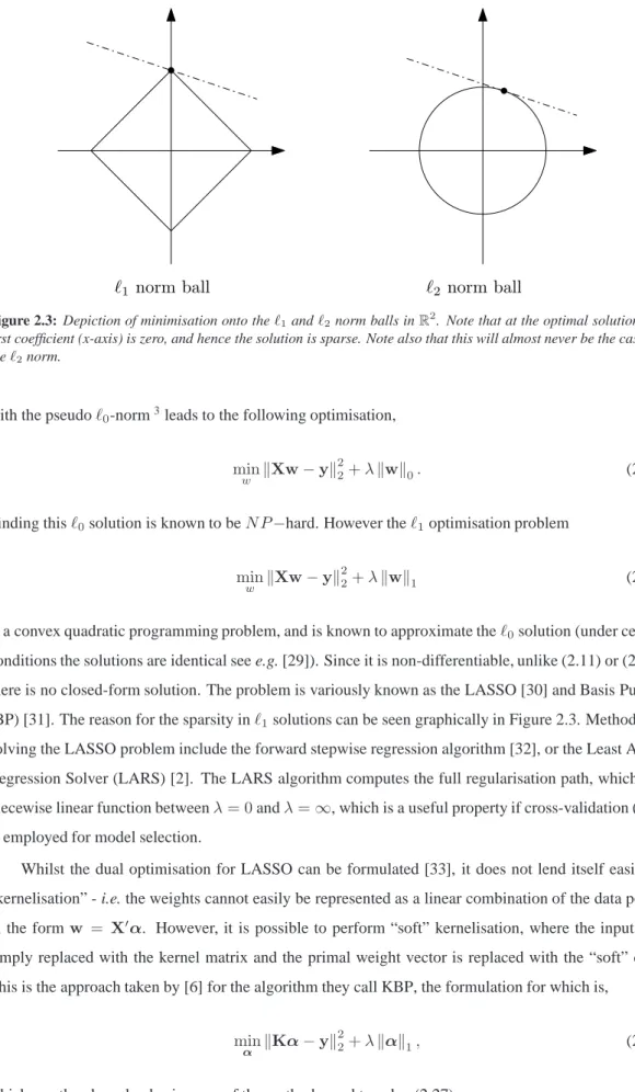
Figure 2.3: Depiction of minimisation onto theℓ1andℓ2norm balls inR2. Note that at the optimal solution, the
first coefficient (x-axis) is zero, and hence the solution is sparse. Note also that this will almost never be the case for theℓ2norm.
with the pseudoℓ0-norm3leads to the following optimisation, min
w kXw−yk
2
2+λkwk0. (2.26)
Finding thisℓ0solution is known to beN P−hard. However theℓ1optimisation problem min
w kXw−yk
2
2+λkwk1 (2.27)
is a convex quadratic programming problem, and is known to approximate theℓ0solution (under certain
conditions the solutions are identical see e.g. [29]). Since it is non-differentiable, unlike (2.11) or (2.22), there is no closed-form solution. The problem is variously known as the LASSO [30] and Basis Pursuit (BP) [31]. The reason for the sparsity inℓ1solutions can be seen graphically in Figure 2.3. Methods for
solving the LASSO problem include the forward stepwise regression algorithm [32], or the Least Angle Regression Solver (LARS) [2]. The LARS algorithm computes the full regularisation path, which is a piecewise linear function betweenλ= 0andλ=∞, which is a useful property if cross-validation (CV) is employed for model selection.
Whilst the dual optimisation for LASSO can be formulated [33], it does not lend itself easily to “kernelisation” - i.e. the weights cannot easily be represented as a linear combination of the data points in the formw = X′α. However, it is possible to perform “soft” kernelisation, where the inputs are simply replaced with the kernel matrix and the primal weight vector is replaced with the “soft” dual. This is the approach taken by [6] for the algorithm they call KBP, the formulation for which is,
min
α kKα−yk
2
2+λkαk1, (2.28)
which can then be solved using any of the methods used to solve (2.27). 3Theℓ
2.1.8
Classification
This Section will introduce methods for classification - i.e. where we want to separate our data into two or more classes. The most obvious way to do this is to create a discriminant function, and as such two methods will be introduced for creating such functions: Fisher Discriminant Analysis (FDA) and the margin-based approach of the Support Vector Machine (SVM). Following on from this two further algorithms will be presented which are based on the notion of boosting - Adaptive Boosting (AdaBoost) and Linear Programming Boosting (LPBoost) - and show how they are related to the margin maximisation principle of the SVM but also in the case of LPBoost to the LASSO approach described earlier.
Preliminaries
Assume we have a sampleS containing examples x ∈ Rn and labelsy ∈ {−1,1}. As before let
X= (x1, . . . ,xm)′be the input vectors stored in matrixXas row vectors, andy= (y1, . . . ,ym)′be a
vector of outputs, where′denote the transpose of vectors or matrices. For simplicity it will be assumed that the examples are already projected into the kernel defined feature space, so that the kernel matrixK has entriesK[i, j] =hxi,xji.
2.1.9
Loss functions for classification
Before going on to give specific examples of learning algorithms for classification, as with the regression case it is worth introducing the different loss functions that are commonly used for classification. Again there is a focus on convex functions, as these lead to optimisation problems that can (in general) be solved exactly. Perhaps the simplest loss function for classification is the zero-one loss, defined as,
L= 0 if yi= sgn(f(xi)) 1 otherwise. (2.29)
If the output of the classifier can be considered a confidence level, it may make sense to penalise larger errors more. A simple modification of the zero-one loss leads to the hinge loss,
L= 0 if yif(xi)≥1 1−yif(xi) otherwise (2.30)
wheref(xi)∈R. This in turn closely resembles the logistic loss, defined as
L= log (1 + exp (−yif(xi))). (2.31)
The square loss, which is closely related to the square loss for regression, and is defined as,
Finally, the linear loss, which relates to a Laplace noise model as it did for regression, is defined as,
L=|1−yif(xi)|. (2.33)
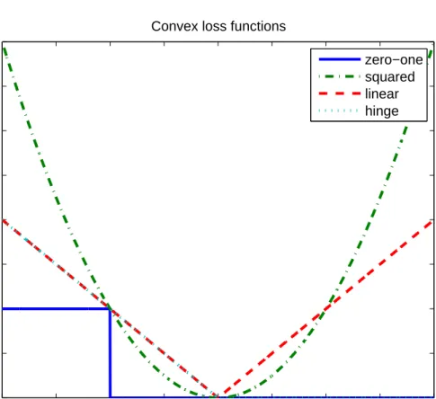
The relations between these loss function can be seen graphically in Figure 2.4. These loss functions
−1 −0.5 0 0.5 1 1.5 2 2.5 3 0 0.5 1 1.5 2 2.5 3 3.5 4 Margin value Loss
Convex loss functions
zero−one squared linear hinge
Figure 2.4: Some examples of convex loss functions used in classification. Note that the hinge loss follows the linear
loss for margin values less than 1, and is zero otherwise. Also note that the hinge loss is a convex upper bound on the zero-one loss.
will play an important role in the rest of the discussion on classification. I will introduce FDA and its kernel equivalent, before showing how this can be cast as a convex optimisation problem using the square loss or the logistic loss.
Fisher Discriminant Analysis
We first review Kernel Fisher Discriminant Analysis (KFDA) in the form given by [3]. The Fisher discriminant chooseswto solve the following optimisation problem
max w
wX′yy′Xw
whereBis a matrix incorporating the label information and the balance of the dataset as follows:
B=D−C+−C−
whereDis a diagonal matrix with entries
Dii = 2m−/m ifyi= +1 2m+/m ify i=−1
andC+andC−are given by
C+ij = 2m−/(mm+) if y i= +1 =yj 0 otherwise C−ij = 2m+/(mm−) if yi=−1 =yj 0 otherwise
Note that for balanced datasetsB will be close to the identity matrixI. The motivation for this choice is that the direction chosen maximises the separation of the means of each class scaled by the variances in that direction.
To solve this problem in the kernel defined feature spaceFwe first need to show that there exists a linear expansionw =Pm
i=1αixiof the primal weight vectorw[34, 3]. This leads to the following
optimisation problem: ρ= max α α′XX′yy′XX′α α′XX′BXX′α (2.35) = max α α′Kyy′Kα α′KBKα = max α α′Qα α′KRα (2.36)
whereQ=Kyy′KandR=BK. The bias termbmust be calculated separately, and there is no fixed way to do this. The most common method is to adjustbsuch that the decision boundary bisects the line joining the two centres of mass,
b=−0.5y′Xw
=−0.5y′Kα (2.37)
The classification function for KFDA is then,
f(xi) = sgn(hw,xii+b)
= sgn(K[:, i]′α+b), (2.38)
be solved. Some algebra shows that it can be solved as the generalised eigenproblemQα=λKR, by selecting theαcorresponding to the largest generalised eigenvalueλ, or in closed form as given by [3],
α=R−1y. Note thatRis likely to be singular, or at best ill-conditioned, and so a regularised solution
is obtained by substitutingR = R+µI, whereµis a regularisation constant. This is equivalent to imposing anl2penalty on the primal weight vector.
However, it has been shown [35, 36] that it is possible to exploit the structure of (2.36) to formulate KFDA as a quadratic program. This is reviewed below.
Convex Fisher Discriminant Analysis
First note that any multiple ofαis also a solution to (2.36). One can further use the observation that the matrixQis rank one. This means thatα′Kycan be fixed to any non-zero value, e.g.2. By minimising the denominator, the following quadratic programme results,
min
α α
′KRα
s.t. α′Ky= 2. (2.39)
Casting the optimisation problem (2.36) as the convex optimisation problem (2.39) gives several advan-tages. Firstly, for large sample sizem, solving the eigenproblem is very costly due to the size ofQand R. The convex formulation also avoids invertingRin the closed form solution which can be unstable. It is also possible to introduce sparsity into theαsolutions through the use of a different regularisation operator. Finally, it will enable the extension of the formulation naturally to multiple views, which is not easily done otherwise (see Section 3.5.2 in the following Chapter). However the unintuitive matrixB still remains in this formulation. Using the fact that KFDA minimises the variance of the data along the projection, whilst maximising the separation of the classes, it is possible to proceed by characterising the variance within a vector of slack variablesξ∈Rn. The variance can then be directly minimised as follows, min α,ξ L(ξ) +µP(α) s.t. Kα+1b=y+ξ ξ′ec= 0 for c= 1,2, (2.40) where eci = 1 ifyi=c 0 otherwise.
L(·),P(·)are the loss function and regularisation functions respectively as follows,
L(ξ) =kξk22, (2.41)
P(α) =α′Kα; (2.42)
where: the first constraint forces the outputs onto the class labels whilst minimising their variance; the second constraint ensures that the label mean for each class is the label for that class, i.e. for±1labels, and the average distance between the classes is two. It has been shown by [35] that any optimal solution
αof (2.40) is also a solution of (2.39). Note that now the bias term is explicitly in the optimisation, and therefore does not need to be calculated separately. The formulation (2.40) has appealing properties that will be used later.
2.1.10
Maximum Margin classification
Geometrically speaking, a maximum-margin hyperplane is a hyperplane that separates two sets of points such that it is equidistant from the closest point in each set and is perpendicular to the line joining the two points. In ML, the concept of large margins encompasses many different approaches to the classification of data from examples, including boosting, mathematical programming, neural networks, and SVM. The key fact is that it is the margin (which can be viewed as a confidence level) of a classification rather than a raw training error that is used when training a classifier [37]. This is known as the hard margin SVM, in which the marginγis maximised as follows,
min
w,b,γ −γ (2.43)
s.t. yi(hw, φ(xi)i+b)≥γ, i= 1, . . . , m
kwk22= 1.
Note that this is equivalent to using the hinge loss defined in Equation (2.30). Cortes and Vapnik [38] modified the maximum margin idea (also known as hard margin) to allow for mislabeled examples. In the absence of a hyperplane that can split the positive and negative examples, the soft margin method chooses a hyperplane that splits the examples as cleanly as possible, while still maximizing the distance to the nearest cleanly split examples. The method introduces slack variables,ξi, which measure the
degree of misclassification of the pointxi. The objective function is then increased by a function which
penalises non-zeroξi, and the optimisation becomes a trade off between a large margin and a small error
penalty. The 2-norm soft margin SVM is defined as the following optimisation problem
min w,b,γ,ξ −γ+Ckξk 2 2 (2.44) s.t. yi(hw, φ(xi)i+b)≥γ−ξi, i= 1, . . . , m kwk22= 1
where the parameterC controls the trade-off between maximising the margin and the size of the slack variables. The resulting algorithm is robust to noise in the data but not sparse in its solutions. In order to enforce sparsity, theℓ1norm is used once again, giving the 1-norm soft margin SVM,
min
w,b,γ,ξ −γ+Ckξk1 (2.45)
s.t. yi(hw, φ(xi)i+b)≥γ−ξi, i= 1, . . . , m
kwk22= 1.
ξi≥0, i= 1, . . . , m.
The dual of this optimisation problem can then be derived, giving us the kernel formulation,
min α m X i,j=1 αiαjyiyjκ(xi, xj) (2.46) s.t. m X i=1 αiyi= 0, m X i=1 αi= 1,and 0≤αi≤C, i= 1, . . . , m
The SVM in this form can be solved by quadratic programming, or alternatively via iterative methods such as the Sequential Minimal Optimisation (SMO) algorithm [39].
2.1.11
Boosting
The term boosting describes any meta-algorithm for performing supervised learning, in which a set of “weak learners” create a single “strong learner”. A weak learner is defined to be a classifier which is only slightly correlated with the true classification (i.e. slightly better than chance). By contrast, a strong learner is strongly correlated with the true classification [40].
Boosting algorithms are typically iterative, incrementally adding weak learners to a final strong learner. At every iteration, a weak learner learns the training data with respect to a distribution. The weak learner is then added to the current strong learner. This is typically done by weighting the weak learner in some manner, which is typically related to the weak learner’s accuracy. After the weak learner is added to the strong learner, the data is reweighted: examples that are misclassified gain weight and examples that are classified correctly lose weight. Thus, future weak learners will focus more on the examples that previous weak learners misclassified.
Adaboost
AdaBoost is the best known example of a boosting algorithm [41]. Without a-priori knowledge, small decision trees, or decision stumps (decision trees with two leaves) are often used. The algorithm works
by iteratively adding in the weak learner that minimises the error with respect to the distributionDtat
steptover the weak learners,
h(t) = arg min hj∈H ǫt= m X i=1 Dt(i)[yi=6 hj(xi)], (2.47)
and then updating the distribution by using the weighted error rate of the classifierhj,
αt= 1 2log 1−ǫt ǫt (2.48) as follows, Dt+1(i) = Dt(i) exp (−αiyiht( xi)) Z (2.49)
whereZis a normalisation constant to ensure thatPm
i=1Dt+1(i) = 1.
The paper [42] describes how the original [41] AdaBoost methods can be extended to the multiclass case4. One of the approaches taken, known as AdaBoost.MH, uses the Hamming loss of the hypotheses
generated fromℓorthogonal binary classification problems. The Hamming loss can be regarded as an average of the error ratehon theseℓbinary problems. Formally, for each weak hypothesish:X→2Y,
and with respect to a distributionD, the loss is
1
ZE(x,Y)∼D[|h(x)∆Y|], (2.50) where∆denotes the symmetric difference, and the leading1/Zensures that values lie in [0,1].
The resulting algorithm, called AdaBoost.MH, maintains a distribution over examplesiand labels ℓ. On roundt, the weak learner accepts such a distributionDtand the training set, and generates a weak
hypothesisht:X×Y→R. This reduction leads to the choice of final hypothesis, which is
H(x, ℓ) = sgn T X t=1 αtht(x, ℓ) ! . (2.51)
The algorithm for AdaBoost.MH is given in Algorithm 1,
Theorem 2.1.1. The reduction used to derive this algorithm implies a bound on the Hamming loss of the final hypothesis:
E(H)≤
T
X
t=1
Zt (2.52)
In the binary classification problem, the goal is to minimise
Zt=
X
i,ℓ
Dt(i, ℓ) exp(−αtY{i,ℓ}ht(xi, ℓ)) (2.53)
Algorithm 1 AdaBoost.MH: A multiclass version of AdaBoost based on Hamming Loss Given training examples(x1, Y1), . . .(xm, Ym), Yi ∈ {+1,−1}ℓ, number of iterationsT
InitialiseD0(i, ℓ) =m1T
fort= 1. . . Tdo
pass distributionDtto weak learner
get weak hypothesisht:X×Y→R
chooseαt(based on performance ofht)
update
Dt+1(i, ℓ) =Dt(i, ℓ) exp(−αtY{i,ℓ}ht(xi, ℓ))/Zt
whereZtis a normalisation factor chosen so thatDt+1will be a distribution
end for
Output final hypothesis:H(x, ℓ) = sign(PT
t=1αtht(x, ℓ))
on each round, wherei= 1. . . mandℓ= 1. . . k(mis the number of examples andkis the number of classes). Since eachhtis required to be in the range−1,+1, eachαtis chosen as follows,
αt= 1 2log 1 +r t 1−rt (2.54) where rt= X i,ℓ Dt(i, ℓ)Y{i,ℓ}ht(xi, ℓ) (2.55) This gives Zt= q 1−r2 t (2.56)
and the goal of the weak learner becomes maximisation of|rt|. The quantity(1−rt)/2is the weighted
Hamming loss with respect toDt.
To relate AdaBoost to the previous discussion of loss functions in Section 2.1.9, the statistical viewpoint is that boosting can be seen as the minimisation of a convex loss function over a convex set of functions [43]. Specifically, the loss being minimized is the exponential loss
L=
m
X
i=1
exp(−yiH(xi)) (2.57)
whereH(xi) =PTt=1f(xi)is the final hypothesis.
Linear Programming Boosting (LPBoost)
Referring back to the 1-norm soft margin SVM in Equation (2.45), it is possible to perform the same optimisation using the weak hypothesis matrixH, whereH = P
y′(φ(x) +b). This would result in the following optimisation (written in matrix form), min w,γ,ξ −γ+C1 ′ξ (2.58) s.t. Hw≥γ1−ξ, kwk22= 1,
where1is the vector of all ones. Since the number of weak learners in the matrixHis potentially very large, it is logical to enforce sparsity in the primal weight vectorw, which can be done by replacing the ℓ2-norm constraint with anℓ1-norm constraint. This results in the following linear programme,
min w,γ,ξ −γ+C1 ′ξ (2.59) s.t. Hw≥γ1−ξ, 1′w= 1, w≥0, ξ≥0.
The dual of this optimisation can then be formulated as follows,
min
α,β β (2.60)
s.t. H′α≤β1, 1′α= 1, 0≤α≤C1,
with dual variablesα andβ, and the box constraints on theα variables are due to the primal slack variablesξ.
The paper by [5] describes an efficient algorithm called LPBoost mimics a simplex based method known as column generation in order to solve the optimisation problem (2.60). The simplex algorithm is a method for finding the numerical solution of the linear programming problem, first introduced by George Dantzig [44]. A simplex is a polytope ofn+ 1vertices inndimensions: a polygon on a line, a pyramid on a plane, etc.
The column generation method involves formulating the problem as if all possible weak hypotheses had already been generated, with the resulting labels becoming the new feature space of the problem. The task that is solved by boosting is to construct a learning function within the output space that minimises misclassification error and maximises the (soft) margin. They prove that for the purposes of classifi-cation, minimising the 1-norm soft margin error function is equivalent to optimising a generalisation error bound. The linear programme is efficiently solved using a technique known as column generation. LPBoost has the advantages over gradient based methods (such as AdaBoost) that it converges in a fi-nite number of iterations to a global solution that is optimal within the hypothesis space, and that these
solutions are very sparse.
The paper cites results that demonstrate that LPBoost performs competitively with AdaBoost on a variety of datasets. The authors also demonstrate that the algorithm is computationally tractable. For both small and large datasets, the computation of the weak learners outweighs the linear programme running time, which means that in general the time for LPBoost iterations are in the same order of magnitude as AdaBoost, though slightly higher.
Many linear programs are too large to consider all the variables explicitly. Since most of the vari-ables will be zero in the optimal solution, only a subset of varivari-ables need to be considered. Column generation generates only variables which have the potential to improve the objective function (i.e. neg-ative reduced cost). The problem being solved is split into two problems, known as the master problem and the subproblem. The master problem is the original problem with only a subset of variables, and the subproblem is a new problem created to identify a new variable. The objective function of the subprob-lem is the reduced cost of the new variable with respect to the current dual variables. LPBoost can be proved to converge in a finite number of iterations to a globally optimal solution within the hypothesis space. In the dual form the constraints are the weak learners.
The algorithm proceeds by adding a weak learner, and checking if the linear programme is solved. If not then the weak learner is found that violates the constraints the most. This process is repeated until the linear programme constraints are not violated, which leads to the global optimum solution. LPBoost iterations are typically slower than AdaBoost, but it converges much more quickly. The LPBoost algo-rithm is given in Algoalgo-rithm 2.
Algorithm 2 LPBoost algorithm
Given training examples(x1, y1), . . .(xm, ym), yi ∈ {+1,−1}, upper limit on weightsC
Initialiseα← m11,H←() whileH′α> βdo h←maxh∈HPmi=1yiαihi,· H ← H h
Updateα: Solve Linear Programme:
arg min β
s.t. H′α≤β1,
0<α< C1. end while
Setwto Lagrangian multipliers
Although at first the boosting methods described above seem rather disjoint from the convex meth-ods described under the general loss minimisation and regularisation framework, there are in fact distinct similarities. If one considers that a general ML principle is to minimise the regularised empirical loss:
min
α L+P(α), (2.61)
regularisation with differening loss functions (hinge loss and quadrtic loss respectively), and between regularised forms of AdaBoost[45] (exponential loss) and the SVM (hinge loss). We can also see the relation between KRR and the convex formulation of KFDA given in Section 2.1.9 where the differences are only in the constraints. See for example [46, 47, 48] for recent discussions of this issue.
2.1.12
Subspace Methods
In standard single view subspace learning, a parallel can be drawn between subspace projections that are independent of the label space, such as Principal Components Analysis (PCA), and those that incorporate label information, such as Fisher Discriminant Analysis (FDA). PCA searches for directions in the data that have largest variance and project the data onto a subset of these directions. In this way a lower dimensional representation of the data is obtained that captures most of the variance. PCA is an unsupervised technique and as such does not include label information of the data. For instance, given 2-dimensional data from two classes forming two long and thin clusters, such that the clusters are positioned in parallel and very closely together, the total variance ignoring the labels would be in the lengthwise direction of the clusters. For classification, this would be a poor projection, because the labels would be evenly mixed. A much more useful projection would be orthogonal to the clusters, i.e. in the direction of least overall variance, which would perfectly separate the two classes. We would then perform classification in this 1-dimensional space. FDA would find exactly this projection.
However if classification is not the goal, but instead the goal is to take a subset of the principal axes of the training data and project both the train and test data into the space spanned by this subset of eigenvectors, the PCA performs this projection by maximising the following criterion,
max
w w
′Σw, (2.62)
s.t. kwk2= 1,
whereΣis the covariance matrix of the centred data - i.e.Σ= 1
m
Pm
i=1(xi−µ)(xi−µ)5. The dual
form of PCA can be formed as follows,
max
α α
′XX′XX′α, (2.63)
s.t. α′XX′α= 1.
Using again the kernel trick, the nonlinear version of PCA known as Kernel Principal Components Analysis (KPCA) [49] is defined as follows,
max
α α
′K2α, (2.64)
s.t. α′Kα= 1.
5The purpose of centering data (transforming data to z-scores) is to remove undesirable fluctuations. Part of the PCA solution
Each of these problems can be solved efficiently as eigenproblems.
2.1.13
Multi-view Learning
Canonical Correlation Analysis (CCA), introduced by Harold Hotelling in 1936 [50], is a method of correlating linear relationships between two sets of multidimensional variables. CCA makes use of two views of the same underlying semantic object to extract a common representation of the semantics. CCA can be viewed as finding basis vectors for two sets of variables such that the correlations between the projections onto these basis vectorsxa = w′aφa(x)andxb = w′bφb(x)are mutually maximised.
Defining the covariance between the two views asΣaband the variance of the views asΣaaandΣbb
respectively, we have the following optimisation problem,
max wa,wb
w′aΣabwb (2.65)
s.t. w′aΣaawa= 1,
w′bΣbbwb= 1.
The major limitation of CCA is its linearity, but the method can be extended to find nonlinear rela-tionships using a the kernel trick once again. Kernel Canonical Correlation Analysis (KCCA) is an implementation of this method that results in a nonlinear version of CCA. Each of the two views of the data are projected into distinct feature spaces such thatwa =X′aαaandwb=X′bαb, before performing
CCA in the new feature space. The dual form of CCA is
max αa,αb α′aXaX′aXbX′bαb (2.66) s.t. α′aXaX′aXaX′aαa = 1, α′bXbX′bXbX′bαb= 1, (2.67)
which leads to the kernelised form, KCCA
max
αa,αb
α′aKaKbαb (2.68)
s.t. α′aK2aαa = 1,
α′bK2bαb= 1,
whereKaandKbare the kernel matrices of the two views.
There have been several successful experimental applications of KCCA on bilingual text corpora, firstly by [51] and later by [52]. In the latter study the authors compare the performance of KCCA with alternative retrieval method based on the Generalised Vector Space Model (GVSM), which aims to capture correlations between terms by looking at co-occurrence information. Their results show that
![Figure 2.2: Structural Risk Minimisation (adapted from [19]). The principle is to find the optimal function f ∗ that satisfies the trade-off between low capacity and low training error](https://thumb-us.123doks.com/thumbv2/123dok_us/1456249.2694838/24.892.166.769.107.1148/figure-structural-minimisation-principle-function-satisfies-capacity-training.webp)