Autonomous Clustering Using Rough Set
Theory
Charlotte Bean
Warwick Medical School University of Warwick Coventry. CV4 7AL. UK [email protected]
Chandra Kambhampati
Department Computer Science University of Hull
Hull. HU6 7RX. UK [email protected]
Abstract – This paper proposes a clustering technique that minimises the need for subjective
human intervention and is based on elements of rough set theory. The proposed algorithm is
unified in its approach to clustering and makes use of both local and global data properties to
obtain clustering solutions. It handles single-type and mixed attribute data sets with ease and
results from three data sets of single and mixed attribute types are used to illustrate the
technique and establish its efficiency.
Index Terms – Rough set theory, data clustering, knowledge-oriented clustering, autonomous
I. INTRODUCTION
Recent years have seen a rapid growth in the volume and complexity of electronic data being
gathered and stored. As a result of this increase, the task of extracting meaningful knowledge in the
form of patterns, relationships and groupings to be used in applications such as decision support,
prediction and taxonomy has become arduous and essential. Furthermore, the need to discover
underlying data structures in mixed attribute data calls for efficient data analysis with minimal human
Cluster analysis is one such technique that is used to reveal characteristics of underlying patterns in
data. It extracts inherent groupings of homogeneous points from heterogeneous data and although
there is no agreed bench-mark definition for the terms ‘cluster’, ‘class’ and ‘group’, they intuitively
describe collections of data points with natural homogeneity. Agglomerative hierarchical clustering
and iterative partitional clustering are two major categories of clustering algorithm that may be cast
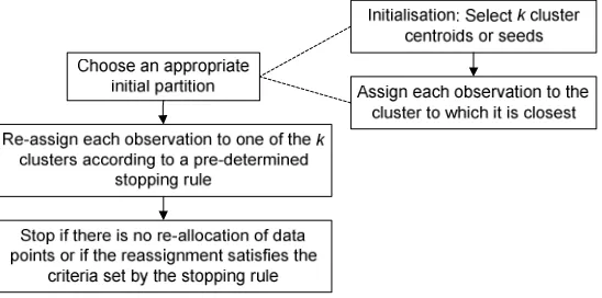
[image:2.595.143.476.261.392.2]into a single algorithmic framework as shown in figs. 1 and 2.
Figure 1: Agglomerative Hierarchical Clustering Framework
Figure 2: Iterative Partitional Clustering Framework
Agglomerative hierarchical clustering [1]-[10] imposes a hierarchical decomposition on a dataset
through the iterative fusion of points and clusters and a final clustering is determined according to
some pre-determined cut-off criterion. Partitional algorithms, including k-means [5],[7],[8],[11]-[16]
and fuzzy c-means (FCM) [17]-[22], follow an iterative optimisation strategy for partitioning a
[image:2.595.180.454.434.570.2]or an initial partition and the successive swapping of data points determines a locally optimal partition.
The FCM methodology differs only in the sense that points are enabled to have a degree of
membership to all clusters. Both categories of clustering technique have advantages and
disadvantages. Hierarchical clustering has an obvious benefit in that it does not require the number of
clusters to be determined a priori, however there is a trade-off in the need to select a termination point
for the algorithm.
Although structurally varied, the two categories of clustering algorithm discussed above share the
common property of relying on local data properties to reach an optimal clustering solution, which
carries the risk of producing a distorted view of the data structure. Rough set theory (RST),
introduced by Pawlak [23]-[26], moves away from this local dependence and focuses on the idea of
using global data properties to establish similarity between objects in the form of coarse and
representative patterns. The rigorous framework of RST is provided by a well-defined indiscernibility
relationship that classifies objects into classes on the basis of perceived differences from an initial
knowledge source and its aim is not to perform exploratory data analysis, but to establish similarities
that are evident in the raw data. In terms of its role as a set theoretical tool, RST is often compared to
fuzzy set theory (FST) with the argument that the two are competing notions. Upon investigating this
view, Dubois and Prade [27] suggested that they are in fact mathematical tools with a different
purpose. Whereas FST deals with the concept of vagueness in the boundary of a sub-class of a set,
RST focuses on coarseness of knowledge within the set itself. It is this notion of coarseness teamed
with the ability to obtain meaningful knowledge from uncertain and incomplete data that makes RST a
valuable tool for extracting relationships from real-world data. Since both cluster analysis and rough
set theory form data groupings, the conceptual link between the techniques is evident [28],[29].
However, the fact that cluster analysis is an exploratory tool used to reveal underlying groupings
discovering ‘possible’ data clusterings with a view to assessing them on the basis of global
information inherent in the data [30]. Early attempts at combining concepts from both techniques
have led to a hierarchical type clustering algorithm called knowledge-oriented clustering [29] in which
a modification procedure allows for the simplification of knowledge. This process of knowledge
simplification is not incorporated in the traditional hierarchical clustering techniques.
This paper proposes an autonomous methodology for extracting knowledge and relationships from
mixed attribute data in the form of coarse clusters which reflect important global properties of the
data. The resultant clustering technique is presented as a simple algorithm and modified tools from
rough set theory are used to form the classes. By virtue of the fact that rough set theory reflects global
data properties, the clustering solution is unaffected by local discrepancies. This then has the
advantages of (a) avoiding the generation of too many small and unrepresentative clusters and (b)
leading to a coarse clustering of the universe. Furthermore, the reliance of the traditional clustering
techniques on local optimality paves the way for a number of different clustering solutions and scope
for distorted results.
The proposed algorithm also eliminates the need for subjectivity in obtaining a representative
number of final clusters and an ‘optimal’ clustering solution is determined according to the
convergence of a well-defined accuracy measure. Procedures to determine data partitionings and
cluster modifications are developed with an emphasis on minimising the level of computational
complexity in order to obtain optimal clusters efficiently. Section II provides a preliminary overview
of rough set theory followed by an introduction to the knowledge-oriented algorithm in section III.
This section incorporates a break-down of the generic clustering procedure and provides a detailed
discussion of the key steps. Section IV introduces the proposed autonomous knowledge-oriented
clustering algorithm and Section V provides a detailed demonstration of the algorithm on real and
II. PRELIMINARIES
The popularity of rough set theory as a tool for handling uncertainty in data has risen since its
introduction in the early 1980s and it has been used successfully in a number of applications such as
data mining, knowledge discovery and decision making [23],[28]-[30]. Its role in knowledge-oriented
clustering will become apparent in the next section but a preliminary overview of the main rough set
concepts will be given here.
Definition 1: Information System
An information system is defined as a family of sets AAAA=(U,A) where Uis a non-empty universe of
objects and A is a finite non-empty set of attributes such that ∀a∈A,a:U→Va, where V is the value a
set of a.
Definition 2: Decision System
Let U be a finite universe of objects and A a finite set of attributes. A decision system is the family of
sets AAAA=(U,A∪{d})such thatd∉Ais a decision attribute and members of A are referred to as
condition attributes
Definition 3: B-Indiscernibility Relation
Let AAAA=(U,A)be an information system. Given a set of attributes B⊆A, classes are formed
according to a B-indiscernibility relation
)} ' ( ) ( , :
' , { )
(B x x U a B a x a x
IndA = ∈ ∀ ∈ = (1)
which induces a partitioning of the universe U according to the attribute set B. The resultant classes
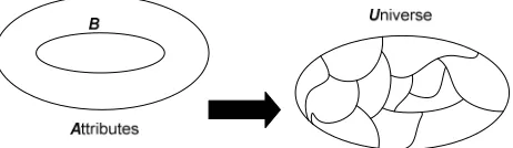
The B-indiscernibility relation is a mathematical equivalence relation that partitions U into a finite
[image:6.595.196.427.192.259.2]number of disjoint equivalence (indiscernibility) classes [x]B as depicted in fig. 3 below.
Figure 3: Partitioning of a Universe, U
Thus, any set X ⊆U can be approximated solely on the basis of information in B⊆ A by
constructing a B-lower approximation and B-upper approximation of X defined respectively as:
Definition 4: B-Lower and Upper Approximations
Let AAAA=(U,A) be an information system and IndA(B)an indiscernibility relation placed on universe
U with respect to the attribute set B⊆A. For a given set X ⊆Ua B-lower approximation of X is
defined as:
} ]
[ :
{x x X
X
B = B ⊆ (2)
and a B-upper approximation of X is defined as
≠ ∩
= x x X
X
B { :[ ]B Ø} (3)
The lower approximation consists of objects that definitely belong to X and the upper approximation
contains objects that possibly belong to X. Consequently, X is classified as a rough set if its
B-boundary region, BNB(X)=BX −BX, is non-empty. In other words, there is a region of uncertainty
degree of overlap between the indiscernibility class [x]B and the rough set X. In this manner,
classifications maintain a global sense of knowledge.
III. KNOWLEDGE-ORIENTEDCLUSTERING:GENERICFRAMEWORK
The generic clustering framework (see figs. 1 and 2) shows how points are traditionally assigned to
clusters according to the two categories of clustering. Although the two procedures are distinct in both
their algorithmic construction and the premise upon which final clusters are obtained, they both rely
on local data properties to refine clustering formations. In the context of hierarchical clustering, this is
through the calculation of distances between clusters whereas the use of local optimality in partitional
clustering leads to the final clustering solution. Without doubt, the two techniques have achieved
success in a range of applications [5],[7],[10],[16] but by extracting selected useful properties of the
algorithms and teaming them with tools from RST, it is possible to overcome some of the drawbacks
associated with these traditional methods through the use of knowledge-oriented (K-O) clustering.
The algorithmic framework of K-O clustering is similar to that of agglomerative hierarchical
clustering (fig. 1). However, the main clustering tool is a form of indiscernibility relation taken from
rough set theory. In using a simple algorithmic framework, K-O clustering is computationally
efficient. Furthermore, the combined use of tools from hierarchical clustering and rough set theory
allows clusters to be formed using both local and global properties of the data. The algorithm to be
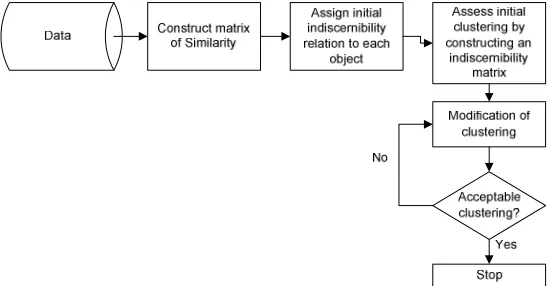
Step 1:Construct a matrix of similarities S={s(xi,xj)} between all pairs of objects
Step 2: Assign an initial indiscernibility relation R to each object in the universe. Pool information i
to obtain an initial clustering U R.
Step 3: Construct an indiscernibility matrix Γ={γ(xi,xj)} to assess the clustering U R.
Step 4: Modify clustering according to a modified indiscernibility relation Rimod to gain a modified
clustering U Rmod.
[image:8.595.164.439.346.489.2]Step 5: Repeat steps 3 and 4 until a stable clustering is obtained.
Figure 4: The Knowledge-Oriented Clustering Algorithm
The notions of similarity and indiscernibility will be introduced and discussed in section 3.1 followed
by a detailed look at the idea of initial clustering in a generic knowledge-oriented clustering
framework in section 3.2.
3.1 Similarity and Indiscernibility
Knowledge-oriented clustering is under-pinned by the construction of two key symmetric matrices;
similarity S={s(xi,xj)}and indiscernibility Γ={γ(xi,xj)}. They respectively control the local and
S is calculated once in the initialisation stage of the algorithm (step 1) whereas the indiscernibility
matrix Γ is updated iteratively (step 3) until convergence to a final clustering solution is achieved.
The re-calculation of the indiscernibility matrix at each iteration reflects updated global knowledge of
the data whereas the single similarity matrix displays inherent local distances between points.
The local properties of points depend on how similar they are to each other, thus the form of the
similarity matrix S is dependent on the distance measure chosen to determine similarity
) , (xi xj
s between pairs of objects. Most clustering algorithms are designed to deal solely with
numerical attributes, however much of the data collected consists of a mixture of both numerical and
categorical attributes (e.g. medical data sets). Thus there is a need for a measure which can take into
account the mixed nature of the data and a combined similarity measure of the following form is
suggested: − + − = ) , ( max ) , ( 1 ) , ( max ) , ( 1 ) , ( , , j i cat j i j i cat cat j i num j i j i num num j i x x s x x s k k x x s x x s k k x x s (5)
where xi,xj are objects in a universe U, k(=knum +kcat)is the total number of attributes, snum is the
similarity measure for numerical data and scatis the similarity measure for categorical data and is,
essentially, the Hamming distance.
The Hamming distance is an appropriate scat measure [31] but the choice of a suitable snum measure
is more difficult due to the nature of the data and the wide selection of possible measures. The
Euclidean Distance measure is well-established and popular, being used in a variety of statistical
fact that the Euclidean distance is scale-invariant can lead to distorted results. Although this can in
some sense be rectified by standardising the data, it should be remembered that this process can itself
affect the clustering solution. Another alternative is to use the Mahalanobis distance. This measure
takes into account the covariance structure of the attributes and acknowledges the fact that significant
correlations between attributes may influence the final result. Again, this cannot be applied in all
circumstances since it relies on the assumptions of normality and homoscedacity in the attributes. It
has been suggested by Manly [32] that the Penrose measure is a more appropriate replacement for the
Mahalanobis distance when dealing with data sets that have less than 100 degrees of freedom. In
summary, the choice of an appropriate snum measure is reliant on a number of factors including the
size and application of the data as well as statistical properties and it must be chosen accordingly to
satisfy the conditions of the given clustering problem.
Global knowledge of the data is represented as the proportion of points that regard each pair of
points in the universe to be indiscernible. The information is displayed in the indiscernibility (or
‘gamma’) matrix Γ which is constructed in step 3 of the algorithm to assess a given clustering
formation and induce modification if necessary. Its entries γ(xi,xj)represent an indiscernibility
degree [31] between each pair of objects xi and xj such that 0≤γ(xi,xj)≤1. The resultant
indiscernibility matrix is defined as follows:
Definition 7: Indiscernibility Matrix
Let AAAA=(U,A) be an information system with non-empty finite universe U ={x1,x2,K,xn}and
attribute set A={a1,a2,K,ak}. For a given clustering of the universe, the indiscernibility matrix
)} , ( {γ xi xj
=
universe to be indiscernible, where the indiscernibility degree γ(xi,xj) for each pair of objects is given by:
∑
∑
∑
= = = + = U k j i dis k U k j i indis k U k j i indis k j i x x x x x x x x 1 1 1 ) , ( ) , ( ) , ( ) , ( γ γ γγ (6)
where = otherwise 0 and if 1 ) ,
( i j k k i k k j
indis k x R x x R x x x γ (7) and = otherwise 0 ) ( not if 1 ) ,
( i j i k j
dis k x R x x x γ (8)
It should be noted that the notion of indiscernibility in this context is more general than the form
outlined in definition 3 of section II and no longer satisfies every property of an equivalence relation.
Def. 3 defines objects to be indiscernible if they possess identical attribute values, whereas a general
form of indiscernibility (see def. 8) allows objects to be regarded as indiscernible if their similarity
value s(xi,xj) exceeds some pre-determined threshold. With this idea in mind, the relations Rk
represent well-defined indiscernibility relations used to partition the universe into classes.
) ,
( i j
indis k x x
γ assesses indiscernibility between xi and xj. It takes the value 1 if xi, xj and xk all lie
in the same indiscernibility class according to the relation Rk. The inclusion of object xk
acknowledges the fact that similarity is measured locally with respect to this point. Conversely
) ,
( i j
dis k x x
γ is equal to 1 if xi and xj are discernible with respect to Rk (i.e. according to relation Rk,
The success of knowledge-oriented clustering hinges on the information obtained from the similarity
and indiscernibility matrices. In the first instance (step 1), the similarity matrix S draws out local
properties of the data in the form of raw distances between points. Since this knowledge forms the
basis of the initial indiscernibility relations Rk used to gain a first partitioning of the universe and
since the initial partitioning should be optimal in the sense that a meaningful and representative
clustering of the data is ultimately attainable, the selection of an appropriate similarity measure is
crucial. On the other hand, the indiscernibility matrix Γ, calculated in step 3 of the algorithm,
displays global knowledge about the positioning of points in the universe which is then used to modify
a given clustering into coarser and more meaningful clusters.
3.2 Initial Clustering of the Data
After initialising the knowledge-oriented clustering algorithm with the calculation of the similarity
matrix S, it is necessary to obtain an initial clustering of the universe (step 2). This step is dependent
on the local knowledge displayed in the similarity matrix and provides a quick overview of the
clustering structure of the data, which can be later modified to form definitive clusters. The initial
clustering should in some sense represent a best possible first clustering. It should be noted, however,
that this notion of optimality does not necessarily imply the initial clustering with the least number of
clusters and since clusters may be subsequently joined but not re-partitioned, it does not increase the
computational burden to obtain a high number of initial clusters.
The initial clustering of the data is governed by key threshold parameters which must be chosen in
order to ensure a true reflection of inherent clustering properties. A failure to do so will lead to a
distorted final clustering. Specifically a set of initial threshold values {Thi}ni=1 is selected to
universe. These are a modified form of indiscernibility that allow two points to belong to the same
indiscernibility class if their similarity value exceeds a pre-determined threshold.
Definition 8: Initial Indiscernibility Relation
Let AAAA=(U,A) be an information system with non-empty finite universe U ={x1,x2,K,xn}and
attribute set A={a1,a2,K,ak}. An initial indiscernibility relation R is assigned to each object in i
the universe as follows:
} , , 2 , 1 , ) , s( : )
,
{(x x U U x x Th j n
Ri = i j ∈ × i j ≥ i = K (9)
where s(⋅ ,⋅) is the similarity measure between two objects and Th is a derived initial threshold value i
for object x . i
i
R induces a partition U Ri of the universe for all i=1,K,n; those objects that are similar to xi
(Pi ={xj:xiRixj})and those objects that are not similar to xi (U−Pi ={xj :not(xiRixj)}). After
obtaining the initial set of partitions,{URi:i=1,2,K,n}, the information is pooled to obtain an overall
initial partitioning of the universe U R, referred to as the initial clustering. The way in which the
partitionings n
i i
R
U } 1
{ = are formed and, thus, the formation of the initial clustering U R is highly
dependent on the choice of the thresholds n
i i
Th} 1
{ = . Hirano and Tsumoto [31] made an attempt to set
these initial threshold values autonomously using the notion of gradient level similarity. This was
achieved by applying a form of Gaussian smoothing to their chosen similarity function in order to
obtain derivative values. Threshold values were selected to correspond to comparably large similarity
decreases. However, not only is this technique computationally intensive, but the notion of using
data sets. A method to overcome these drawbacks in setting the initial threshold values is suggested in
section IV.
IV. KNOWLEDGE-ORIENTEDCLUSTERINGWITHAUTONOMY
Knowledge-oriented clustering algorithms can be framed within a generic algorithmic framework
(fig. 4), but the efficiency and optimality of the algorithm is dependent on the selection of individual
threshold parameters. Not only is this relevant to the initial clustering of the universe, but it is also
true in the modification stages of the algorithm (step 4) where further threshold values determine
updated partitionings of the universe. However, whereas traditional hierarchical clustering algorithms
[1]-[10] rely on subjectivity to determine parameters, it is desirable to develop a set of well-defined
procedures for setting the required thresholds autonomously at each stage of the knowledge-oriented
clustering algorithm, thus ensuring the same (or a highly similar) clustering solution upon applying the
algorithm through independent means to the same data. This section details such procedures within
the generic framework outlined in section III. Section 4.1 introduces a method for obtaining a set of
initial threshold values {Thi}ni=1 which will lead to an optimal initial clustering of the universe, where
optimality is in the sense discussed previously, and sections 4.2 and 4.3 discuss the notion of cluster
modification.
4.1 Autonomous Initial Clustering of the Data
The initial clustering of the universe is a crucial stage in the knowledge-oriented clustering
procedure. If done in an incorrect manner, the subsequent clusterings will not fully reflect inherent
data structures, leading to a distorted and meaningless final clustering. Since the initial partitioning is
achieved by imposing initial indiscernibility relations (9) on the data, which are themselves dependent
meaningful clustering of the universe. A method is suggested here to determine the initial thresholds
autonomously whilst maintaining the key goal of computational efficiency.
In a physical sense, the centre of gravity (CoG) is an imaginary point around which the centre of an
object’s weight lies. Using this idea, points in a plane can be separated into two classes by a line upon
which their CoG lies. For two distinct and equally weighted clusters of points, the line will lie
mid-way between them and naturally as the distinction between clusters becomes more ambiguous, the line
will move up or down to reflect this. In the K-O clustering algorithm, the initial threshold values take
on this role of partitioning the objects into two classes. The closer points lie to the object in question,
the ‘higher’ the threshold line is expected to be. In other words, a sensible positioning of the initial
threshold line is the line upon which the CoG of the points lies. This shall be referred to as the ‘CoG
line’.
x
x x x
x x
x
x x x
x x
x x
x x
[image:15.595.234.383.399.579.2]x x
Figure 5: Centre of Gravity Line
The CoG line of a set of points in the plane is positioned such that the sum of all perpendicular
distances from the points to this line is zero. These calculations may be weighted if the CoG line is
seemingly distorted by outlying points. Following this method, an initial threshold Thi corresponding
to the object xi may be obtained by selecting the similarity value s(xi,xk),k =1,2,K,n, which
(
s x x ws x x)
i nn j
k i j
i, ) ( , ) , 1,2, ,
( 1
L
= −
∑
=
(10)
w is a weighting value that is usually set to 1 but may be set to 2 to raise the CoG line if necessary.
This procedure produces a set of initial threshold values corresponding to each object in the universe
from which the initial partitionings may be obtained. This information is then pooled to obtain the
initial clustering of the universe U R.
4.2 Assessment and Modification of Clusters
As mentioned earlier, the algorithm in the initial step will consist of a relatively high number of
clusters. This is a result of the way in which the initial indiscernibility relations partition the universe.
Specifically, each initial indiscernibility relation Ri imposes a partitioning of the universe U Ri
consisting of two classes. High numbers of initial clusters occur if the relations Ri disagree on which
pairs of points should belong to the same class. For example, for a given information system, if
relation Ri places objects xi and xj in different classes, they will automatically belong to different
clusters in the initial clustering; even if every other indiscernibility relation places them in the same
class. This may be rectified in the later steps of the algorithm using global modification which alters
this and, thus, the need for a high number of clusters. The global modification of any given clustering
is controlled by the indiscernibility matrix Γ={γ(xi,xj)}introduced in the earlier section. Its entries
) , (xi xj
γ assess the indiscernibility degree between each pair of objects in the universe and determine
what proportion of the initial indiscernibility relations regard the two points to be indiscernible. In this
way, the indiscernibility degree between two objects overlooks local discrepancies between
equivalence relations. Modification to the given clustering is then performed using a modified
Definition 9: Modified Indiscernibility Relation
Let AAAA=(U,A) be an information system with non-empty finite universe U ={x1,x2,K,xn}and
attribute set A={a1,a2,K,ak}. Suppose that U R is a given clustering of the universe. The
clustering is modified according to the indiscernibility relation:
R {(xi,xj) U U: (xi,xj) Th , j 1, ,n}
mod
i = ∈ × γ ≥ γ = K (11)
where Thγ is a pre-determined gamma threshold value.
In performing modification, a given clustering U R is adapted to gain a coarser and more
meaningful clustering of the universe U Rmod . As with the initial thresholds, the choice of the
gamma threshold value at each modification step will directly influence the final clustering obtained.
It is therefore imperative that this value is chosen carefully. In previous work, the gamma value has
effectively been hand-picked with a view to assessing the validity of obtained clusterings and allowing
for re-selection of an appropriate value if necessary [29]. This method does provide good clusterings,
however, in keeping with the desire to maintain a high degree of autonomy and computational
efficiency in the algorithm, it is preferable and less cumbersome to select the gamma threshold value
autonomously according to some pre-determined accuracy criterion. A method for achieving this
based on a defined clustering accuracy measure is suggested in section 4.3
4.3 Autonomous Selection of Gamma Thresholds in Cluster Modification
The aim of knowledge-oriented clustering is to use both local and global knowledge to determine the
partitioning of a given data set which, in some sense, represents an ‘accurate’ clustering of the
combination of two distinct accuracy measures; accwithin and accbetween. They respectively represent
within and between-clusters accuracy (as defined in defs. 10 and 11). The within-clusters accuracy
)
(accwithin determines the degree of homogeneity within clusters for a given clustering formation. It is
calculated as the mean (with respect to the number of clusters, K) of the set of standard deviations of
the unique similarity values corresponding to the objects in each cluster. For consistency, the trivial
case of similarity between a point and itself is included. The result is modified to reduce the
occurrence of too many clusters containing just one point (‘one point clusters’). Between-clusters
accuracy (accbetween) is taken as the mean of the minimum distances between each cluster, where the
set of appropriate distances has been reduced to exclude distances between clusters lying at extreme
ends of the clustering space. The aim is to gain a clustering which reflects a high degree of
homogeneity within the clusters and the opposite between the clusters. Due to the nature of the
similarity value (5), lower acc values represent a more accurate clustering.
Definition 10
Let U R={C1,C2,K,CK} be a clustering of the universe U. If a given cluster Ck ,k∈{1,2,K,K},
contains m objects {x1,x2,K,xm}, define the function A( )
k
C :
m x x s C
k C m
i j
m i
j i k
2 1
1
] ) , ( [
) A(
µ
∑∑
> −
=
−
= (12)
where s(xi,xj) represents the similarity between objects x and i x and j
k C
µ is the mean of the
2 1
) ( )
( P
K C A acc
K k
k U
within ×
=
∑
=R (13)
where P is the number of clusters with cardinality 1.
Definition 11
Let U R={C1,C2,K,CK} be a clustering of the universe U. Let d(Ci,Cj) be the minimal distance
between clusters C and i C , where this is calculated as the maximum similarity value between points j
in each cluster for the similarity measure defined in equation (5). Define:
1 , ) 1 (
) , ( 2
1
1 1
> −
=
∑ ∑
−= =+
K K
K
C C d X
K i
K i j
j i
(14)
and let B={d(Ci,Cj):d(Ci,Cj)≥ X}. Between clusters accuracy for the clustering U R is defined
as:
) ( )
( B
acc U
between R =µ (15)
where µ represents the mean value of the set B.
Using definitions 10 and 11, a gamma threshold value can be chosen autonomously according to
Proposition 1
If U R is a given clustering of the universe U and N i i
Th } 1
{ γ = a pre-determined set of possible gamma
thresholds, then the threshold Thγ used to achieve the modified clustering U Rmod is chosen from the
set N
i i
Th } 1
{ γ = to correspond to the minimum accuracy value:
)} ( 9
. 0 ) ( 1 . 0 { min ) ( min
i i
i U i i
U
U between U
within
U acc acc
acc γ γ γ
γ γ
R R
R
R R
+
= (16)
where {URγi}iN=1 are the partitionings generated by the values
N i i
Th } 1
{ γ = respectively.
The modification process is iterated until convergence to a stable acc value is achieved, at which point
the corresponding clustering is deemed to be the final and optimal clustering of the universe with
respect to the defined accuracy value (16).
V. EXPERIMENTALRESULTS
In this section, three data sets are clustered using the above algorithm. In the first instance,
knowledge-oriented clustering with autonomy is used to cluster a small test data set. In section 5.1 a
step-by-step break-down of the procedure, which corresponds to the generic algorithmic framework
stated in fig. 4, is given. The food nutrient data, available in the Agriculture Yearbook [33], is
clustered in section 5.2 as a practical demonstration of the algorithm and section V concludes with an
5.1 Laboratory Generated Data Results
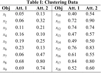
A small test data set, consisting of 18 objects and 2 continuous attributes (table I), was generated in
the department to verify the functionality of the autonomous knowledge-oriented clustering algorithm.
The data set is sufficiently small to enable the workings of the algorithm to be described in an explicit
manner, whilst the clear clustering structure (as seen in fig. 6) highlights the data as a suitable
candidate for any clustering procedure. Through visual analysis of the data plot, three clusters seem
apparent. However, upon applying K-O clustering to the data, a result of four clusters is achieved (fig.
7). This suggests that the use of global modification draws out inherent global data properties which
remain concealed in a locally-dependent algorithm. In order to outline the detailed process of K-O
clustering, a summary of the step-by-step procedure for the data in table I, as stated in fig. 4, is
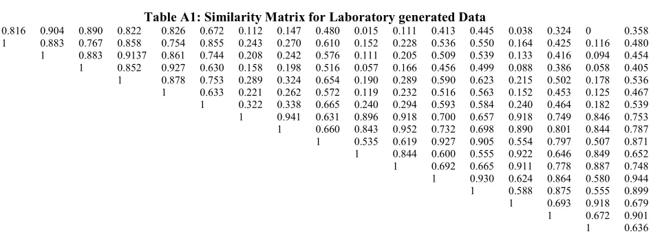
provided below. Upper triangular forms of the symmetric similarity matrix (table A1) and
indiscernibility matrices (tables A2 and A3) for all stages in the algorithm are provided in the
appendix.
Step 1: Construct matrix of similarities between all pairs of objects
The Euclidean distance was selected as an appropriate snum measure for this data and similarity
between objects x1 and x2, s(x1,x2) and objects x1 and x18, s(x1,x18) were calculated as:
where maxs ( , ) 1.0359 ,j num i j =
i x x . Recall that, due to the nature of the similarity measure (5),
similarity values closer to 1 indicate a greater similarity between objects. The complete similarity
matrix is displayed in the appendix (table A1).
Step 2: Assign an initial indiscernibility relation Ri to each object in the universe and pool the
information to obtain an initial clustering U R
Initial threshold values Thi were assigned to each object in the universe using the centre of gravity
method (10) with w = 2. The results for objects x1 and x18 are displayed below:
}} , , , , , , , , , , , { }, , , , , , {{ }} , , , , , , , , , , , { }, , , , , , {{ 17 15 12 11 8 7 6 5 4 3 2 1 18 16 14 13 10 9 18 18 17 16 15 14 13 12 11 10 9 8 7 6 5 4 3 2 1 1 x x x x x x x x x x x x x x x x x x R U x x x x x x x x x x x x x x x x x x R U = = M
where Th1 =0.81632 and Th18 =0.7874. Upon pooling the individual partitionings, the initial
partitioning of the universe U R produced 8 clusters (as shown in fig. 6):
}} { }, , , , , { }, { }, , , , { }, { }, { }, { }, , , , {{ 12 18 16 14 13 10 9 17 15 11 8 7 6 4 5 3 2 1 x x x x x x x x x x x x x x x x x x
U R=
Step 3: Construct an indiscernibility matrix to assess the clustering U R
Using equation (6), the indiscernibility degrees between object x1 and various other objects are
shown below: 42857 . 0 ) , ( and 85714 . 0 ) , ( , 1 ) ,
(x1 x2 = γ x1 x4 = γ x1 x7 =
These results indicate that 100% of the relations assign objects x1 and x2 to the same class whereas
only 42.86% of the relations would place x1 and x7 together.
Step 4: Modify clustering according to a modified indiscernibility relation Rimod to gain a
modified clustering U Rmod
After calculating the complete gamma matrix, the initial clustering was modified with Thγ =0.5. Two
examples of the individual modified partitionings are shown below followed by the modified
clustering of the universe U Rmod :
}} , , , , , , , , , , , , { }, , , , , {{ }} , , , , , , , , , , , { }, , , , , , {{ 17 15 12 11 9 8 7 6 5 4 3 2 1 18 16 14 13 10 mod 18 18 17 16 15 14 13 12 11 10 9 8 7 6 5 4 3 2 1 mod 1 x x x x x x x x x x x x x x x x x x R U x x x x x x x x x x x x x x x x x x R U = = M }} , , , , { }, , , , , , { }, { }, , , , , ,
{{ 1 2 3 4 5 6 7 8 9 11 12 15 17 10 13 14 16 18
mod x x x x x x x x x x x x x x x x x x
U R =
Step 5: Repeat steps 3 and 4 until a stable clustering is obtained
For the data given in table I, convergence to the final solution was obtained after just one iteration
[image:23.595.210.411.553.699.2]and the resulting clusters are displayed in fig. 7.
Table I: Clustering Data
Obj Att. 1 Att. 2 Obj Att. 1 Att. 2
1
x 0.05 0.13 x10 0.40 0.54
2
x 0.06 0.32 x11 0.72 0.90 3
x 0.11 0.21 x12 0.74 0.74
4
x 0.16 0.10 x13 0.47 0.57
5
x 0.19 0.25 x14 0.49 0.50 6
x 0.23 0.13 x15 0.76 0.83
7
x 0.06 0.47 x16 0.61 0.55
8
x 0.68 0.80 x17 0.84 0.80 9
Figure 6: Initial Clusters Figure 7: Final Clusters
5.2 Practical Clustering Demonstration: Food Nutrient Data
The second data set to be considered is a real-world application. The food nutrient data available in
the Agriculture Yearbook (see [33] for details) has been clustered here using K-O clustering both with
and without autonomy [28] and the results displayed below (tables II and III). This classical clustering
data set consists of 27 objects; different types of meat, fish and foul and 5 attributes; food-calories,
protein, fat, calcium and iron (see appendix, table A4). Protein and iron were found to be superfluous
to the clustering [8] so, for the purpose of visualising the final clusters, the results obtained using 3
[image:24.595.119.502.99.244.2]attributes; food-calories, fat and calcium will be discussed.
Table II: Autonomous Clustering Results for Food Nutrient Data
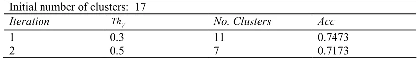
Initial number of clusters: 17
Iteration Thγ No. Clusters Acc
1 0.3 11 0.7473
[image:24.595.97.520.502.562.2]2 0.5 7 0.7173
Table III: Non-Autonomous Clustering Results for Food Nutrient Data
Initial number of clusters: 16 Thstd: 0.11
Iteration Thγ No. Clusters Acc
1 0.5 14 0.7625
2 0.4 9 0.7575
[image:24.595.97.518.603.678.2]Tables II and III display the results of K-O clustering with and without autonomy respectively. The
autonomous algorithm converged after 2 iterations to a final solution of 7 clusters (table II) and the
algorithm without autonomy converged after 3 iterations to a solution of 5 clusters (table III). Since
the algorithmic framework of knowledge-oriented clustering is similar to that of hierarchical
clustering (see fig. 4), these results are compared in table VII to those obtained using four traditional
agglomerative hierarchical clustering techniques; namely complete-linkage, single-linkage,
average-linkage and Ward’s method where the numbers indicate cluster membership. Although the two
knowledge-oriented methods led to different final solutions, the similarities between the resulting
clusters far out-weigh the differences, thus suggesting that both versions of the K-O algorithm have
identified the salient features of the data. Furthermore, autonomous K-O clustering is operated with
minimal subjectivity which guarantees consistent results when applied to the same data by different
users. In contrast, the different methods within the agglomerative hierarchical clustering category
produce different solutions on the same data. A cross-section of the similarity and gamma values
calculated throughout the procedure is provided below (tables IV,V,VI) corresponding to the five
[image:25.595.194.426.522.612.2]numbered objects in fig. 8, where the Euclidean distance was chosen as the snum measure.
Table IV: Similarity Values for Food Nutrient Data
) , (xi xj
s x4 x10 x22 x24 x25
4
x 1 0.8263 0.3863 0.3150 0.0586
10
x 0.8263 1 0.5208 0.4578 0.1286
22
x 0.3863 0.5208 1 0.9186 0.5124
24
x 0.3150 0.4578 0.9186 1 0.5008
25
x 0.0586 0.1286 0.5124 0.5008 1
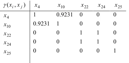
Table V: Gamma Values at Iteration 1 for Food Nutrient Data
) , (xi xj
γ x4 x10 x22 x24 x25
4
x 1 0.6667 0 0 0
10
x 0.6667 1 0 0 0
x22 0 0 1 1 0.1429
24
x 0 0 1 1 0.1429
25
[image:25.595.185.430.638.729.2]Table VI: Gamma Values at Iteration 2 for Food Nutrient Data
) , (xi xj
γ x4 x10 x22 x24 x25
4
x 1 0.9231 0 0 0
10
x 0.9231 1 0 0 0
22
x 0 0 1 1 0
24
x 0 0 1 1 0
25
[image:26.595.115.507.243.745.2]x 0 0 0 0 1
Table VII: Comparison of Clustering Results for Food Data
Object Food Item K-O with Autonomy
K-O without Autonomy
Comp.-Linkage & Ward’s
Single-Linkage
Average-Linkage
1 Braised beef 1 1 1 1 1
2 Hamburger 5 5 2 1 1
3 Roast beef 7 1 1 7 1
4 Beef steak 1 1 1 1 1
5 Canned beef 2 2 2 2 2
6 Broiled chicken 3 2 3 2 2
7 Canned chicken 2 2 2 2 2
8 Beef heart 2 2 2 2 2
9 Roast lamb leg 5 5 2 1 1
10 Roast lamb shoulder 1 1 2 1 1
11 Smoked ham 1 1 1 1 1
12 Roast pork 1 1 1 1 1
13 Simmered pork 1 1 1 1 1
14 Beef tongue 2 2 2 2 2
15 Veal cutlet 2 2 2 2 2
16 Baked bluefish 3 2 3 2 2
17 Raw clams 3 3 3 3 3
18 Canned clams 3 3 3 3 3
19 Canned crabmeat 3 2 3 2 2
20 Fried Haddock 2 2 3 2 2
21 Broiled mackerel 2 2 2 2 2
22 Canned mackerel 6 3 3 6 3
23 Fried perch 2 2 2 2 2
24 Canned salmon 6 3 3 6 3
25 Canned sardines 4 4 4 4 4
26 Canned tuna 2 2 2 2 2
27 Canned shrimp 3 2 3 5 3
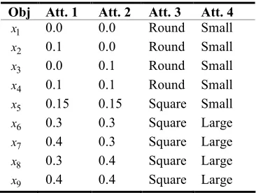
[image:26.595.114.510.246.726.2]5.3 Mixed Attribute Data
In order to establish the effectiveness of the autonomous knowledge-oriented clustering algorithm on
a mixed attribute data set, the small data set shown in table VIII below has been clustered. It consists
of 9 objects and 4 attributes; 2 continuous attributes and 2 categorical attributes, and was originally
[image:27.595.218.401.249.387.2]used by Hirano and Tsumoto [31].
Table VIII: Mixed Attribute Data Set Obj Att. 1 Att. 2 Att. 3 Att. 4
1
x 0.0 0.0 Round Small
2
x 0.1 0.0 Round Small
3
x 0.0 0.1 Round Small
4
x 0.1 0.1 Round Small
5
x 0.15 0.15 Square Small
6
x 0.3 0.3 Square Large
7
x 0.4 0.3 Square Large
8
x 0.3 0.4 Square Large
9
x 0.4 0.4 Square Large
The Similarity matrix S (table A5) was calculated using the Euclidean distance as an appropriate
num
s measure and the Hamming distance as the scat measure. Using the centre of gravity method with
1 =
w , the following initial indiscernibility relations were obtained and led to an initial clustering
R
U of four clusters:
}} , , , { }, , , , , {{ , ,
, 2 3 4 1 2 3 4 5 6 7 8 9
1 U R U R U R x x x x x x x x x
R U = }} , , , , { }, , , ,
{{ 2 3 4 5 1 6 7 8 9
5 x x x x x x x x x
R U = }} , , , , { }, , , , {{ , ,
, 7 8 9 1 2 3 4 5 6 7 8 9
6 U R U R U R x x x x x x x x x
R U = }} , , , { }, { }, , , { },
{{x1 x2 x3 x4 x5 x6 x7 x8 x9
U R=
The algorithm converged with Thγ =0.2 after just one iteration to a final solution of three clusters;
}} , , , { }, { }, , , ,
{{ 1 2 3 4 5 6 7 8 9
mod x x x x x x x x x
appendix (table A6). In contrast to the result obtained by Hirano and Tsumoto [31], autonomous
knowledge-oriented clustering has placed point x5 into a cluster on its own, resulting in three rather
than two final clusters. However, both the raw data (table VIII) and the indiscernibility matrix (table
A6) exhibit a degree of ambiguity surrounding the placement of this point. This suggests that
autonomous K-O clustering has exhibited a greater sensitivity to the inherent data knowledge by
maintaining a one point cluster containing point x5.
VI. CONCLUSIONS AND FUTURE WORK
Cluster analysis is an important exploratory technique for discovering patterns and underlying
structure in data. The aim of clustering is to partition a data set into classes such that within-class
homogeneity is high and between-class homogeneity weak. However, standard clustering techniques,
including agglomerative hierarchical algorithms, K-means clustering and fuzzy c-means clustering,
carry a number of inherent problems that directly influence the clustering solution. In all cases, a high
degree of subjectivity is required to obtain an ‘optimal’ clustering solution. This results in a
non-unified approach to clustering, allowing for different clusters to be obtained when a given technique is
applied to the same data by different people. This puts the optimality of any given solution under
scrutiny in terms of how well it really reflects true underlying data structures. Furthermore, the
standard techniques generally focus on the clustering of single-type attribute data sets (e.g. continuous
attributes) and are unable to cope easily with mixed attribute data. In terms of clustering applications,
such as medical data, this is a major disadvantage.
In order to overcome these problems, this paper has proposed an autonomous knowledge-oriented
clustering algorithm. The algorithmic framework forms clusters autonomously according to some
pre-defined accuracy measure. In this way, the technique is standardised in the sense that multiple
solution. The algorithm handles mixed attribute data with ease and is such that no modification to the
algorithm is needed to move between data sets of different attribute types.
It should be noted that the convergence of the algorithm to an ‘optimal’ solution is governed by the
similarity and indiscernibility matrices which represent local and global knowledge respectively. It is
this, teamed with the algorithm’s standardised approach, that gives knowledge-oriented clustering the
edge over other techniques. By incorporating global knowledge into the procedure, a coarse and
representative clustering of the universe is obtained efficiently.
It was demonstrated that the use of global modification draws out important data properties, which
remain hidden in the standard clustering algorithms, and leads to a representative clustering and it is
hypothesised that the knowledge-oriented clustering procedure may be used to extract ‘optimal’ and
non-ambiguous rules for a decision support system [28]. It remains as further work to assess the
performance of the algorithm in situations of high ambiguity where clusters lie particularly close or
are, indeed, overlapping.
[image:29.595.69.542.481.651.2]APPENDIX
Table A1: Similarity Matrix for Laboratory generated Data
1 0.816 0.904 0.890 0.822 0.826 0.672 0.112 0.147 0.480 0.015 0.111 0.413 0.445 0.038 0.324 0 0.358 1 0.883 0.767 0.858 0.754 0.855 0.243 0.270 0.610 0.152 0.228 0.536 0.550 0.164 0.425 0.116 0.480 1 0.883 0.9137 0.861 0.744 0.208 0.242 0.576 0.111 0.205 0.509 0.539 0.133 0.416 0.094 0.454 1 0.852 0.927 0.630 0.158 0.198 0.516 0.057 0.166 0.456 0.499 0.088 0.386 0.058 0.405 1 0.878 0.753 0.289 0.324 0.654 0.190 0.289 0.590 0.623 0.215 0.502 0.178 0.536 1 0.633 0.221 0.262 0.572 0.119 0.232 0.516 0.563 0.152 0.453 0.125 0.467 1 0.322 0.338 0.665 0.240 0.294 0.593 0.584 0.240 0.464 0.182 0.539 1 0.941 0.631 0.896 0.918 0.700 0.657 0.918 0.749 0.846 0.753 1 0.660 0.843 0.952 0.732 0.698 0.890 0.801 0.844 0.787 1 0.535 0.619 0.927 0.905 0.554 0.797 0.507 0.871 1 0.844 0.600 0.555 0.922 0.646 0.849 0.652 1 0.692 0.665 0.911 0.778 0.887 0.748 1 0.930 0.624 0.864 0.580 0.944 1 0.588 0.875 0.555 0.899 1 0.693 0.918 0.679 1 0.672 0.901 1 0.636
Table A2: Indiscernibility Matrix at Iteration 1 for Laboratory Generated Data
1 1 1 0.857 1 0.714 0.429 0 0 0 0 0 0 0 0 0 0 0
1 1 0.857 1 0.714 0.429 0 0 0 0 0 0 0 0 0 0 0
1 0.857 1 0.714 0.429 0 0 0 0 0 0 0 0 0 0 0
1 0.857 0.833 0.286 0 0 0 0 0 0 0 0 0 0 0
1 0.714 0.429 0 0 0 0 0 0 0 0 0 0 0
1 0.143 0 0 0 0 0 0 0 0 0 0 0
1 0 0 0 0 0 0 0 0 0 0 0
1 0.6 0 1 0.857 0 0 1 0 1 0
1 0.364 0.6 0.7 0.364 0.364 0.6 0.364 0.6 0.364
1 0 0.091 1 1 0 1 0 1
1 0.857 0 0 1 0 1 0
1 0.091 0.091 0.857 0.091 0.857 0.091
1 1 0 1 0 1
1 0 1 0 1
1 0 1 0
1 0 1
1 0
[image:30.595.71.524.116.480.2]1
Table A3: Indiscernibility Matrix at Iteration 2 for Laboratory Generated Data
1 1 1 1 1 1 0 0 0 0 0 0 0 0 0 0 0 0
1 1 1 1 1 0 0 0 0 0 0 0 0 0 0 0 0
1 1 1 1 0 0 0 0 0 0 0 0 0 0 0 0
1 1 1 0 0 0 0 0 0 0 0 0 0 0 0
1 1 0 0 0 0 0 0 0 0 0 0 0 0
1 0 0 0 0 0 0 0 0 0 0 0 0
1 0 0 0 0 0 0 0 0 0 0 0
1 1 0 1 1 0 0 1 0 1 0
1 0 1 1 0 0 1 0 1 0
1 0 0 1 1 0 1 0 1
1 1 0 0 1 0 1 0
1 0 0 1 0 1 0
1 1 0 1 0 1
1 0 1 0 1
1 0 1 0
1 0 1
Table A4: Food Nutrient Data
Object Food Item Calories Protein Fat Calcium Iron
1 Braised beef 340 20 28 9 2.6
2 Hamburger 245 21 17 9 2.7
3 Roast beef 420 15 39 7 2.0
4 Beef steak 375 19 32 9 2.6
5 Canned beef 180 22 10 17 3.7
6 Broiled chicken 115 20 3 8 1.4
7 Canned chicken 170 25 7 12 1.5
8 Beef heart 160 26 5 14 5.9
9 Roast lamb leg 265 20 20 9 2.6
10 Roast lamb shoulder 300 18 25 9 2.3
11 Smoked ham 340 20 28 9 2.5
12 Roast pork 340 19 29 9 2.5
13 Simmered pork 355 19 30 9 2.4
14 Beef tongue 205 18 14 7 2.5
15 Veal cutlet 185 23 9 9 2.7
16 Baked bluefish 135 22 4 25 0.6
17 Raw clams 70 11 1 82 6.0
18 Canned clams 45 7 1 74 5.4
19 Canned crabmeat 90 14 2 38 0.8
20 Fried Haddock 135 16 5 15 0.5
21 Broiled mackerel 200 19 13 5 1.0
22 Canned mackerel 155 16 9 157 1.8
23 Fried perch 195 16 11 14 1.3
24 Canned salmon 120 17 5 159 0.7
25 Canned sardines 180 22 9 367 2.5
26 Canned tuna 170 25 7 7 1.2
27 Canned shrimp 110 23 1 98 2.6
Table A5: Similarity Matrix for Mixed Attribute Data
1 0.9116 0.9116 0.8750 0.5625 0.1250 0.0581 0.0581 0 1 0.8750 0.9116 0.6102 0.1813 0.1250 0.1047 0.0581
1 0.9116 0.6102 0.1813 0.1047 0.1250 0.0581 1 0.6875 0.2500 0.1813 0.1813 0.1250 1 0.5625 0.4923 0.4923 0.4375 1 0.9116 0.9116 0.8750 1 0.8750 0.9116 1 0.9116
1
Table A6: Indiscernibility Matrix for Mixed Attribute Data
1 0.8 0.8 0.8 0.4444 0 0 0 0
1 1 1 0.5556 0 0 0 0
1 1 0.5556 0 0 0 0
1 0.5556 0 0 0 0
1 0.4444 0.4444 0.4444 0.4444
1 1 1 1
1 1 1
1 1
REFERENCES
[1] T. Sǿrensen, “A method of establishing groups of equal amplitude in plant sociology based on similarity of species content and its application to the analyses of the vegetation on Danish commons,” Biologiske Skrifter, 5(4), 1-34, 1948
[2] P. Sneath, “The application of computers to taxonomy,” Journal of General Microbiology, vol. 17, no. 1, 201-226, 1957
[3] R. Sokal and P. Sneath, Principles of Numerical Taxonomy, W.W.Freeman, San Francisco,
1963
[4] J. Ward, “Hierarchical grouping to optimize an objective function,” Journal of the American
Statistical Association, vol. 58, no. 301, 236-244, 1963
[5] M. P. Anderberg, Cluster Analysis for Applications, New York, Academic Press, 1973
[6] M. S. Aldenderfer and R. K. Blashfield, Cluster Analysis, Sage University Paper, Newbury Park, 1984
[7] B. S. Everitt, Cluster Analysis, Cambridge, Edward Arnold, 1993
[8] S. Sharma, Applied Multivariate Techniques, New York, Wiley, 1996
[9] A. K. Jain, M. N. Murty and P. J. Flynn, “Data clustering: a review”, ACM Computing Surveys, vol. 31, no.3, pp. 264 – 323, 1999
[10] R. R.Yegar, “Intelligent control of the hierarchical clustering process”, IEEE Transactions
on Systems., Man and Cybenetics., vol. 30, PART B no. 6, pp. 835 – 845, 2000
[11] E. W. Forgey, Cluster Analysis of Multivariate Data: Efficiency Versus Interpretability of
Classifications, Biometrics, vol. 21, no.3, pp. 768-769, 1965
[12] R. C. Jancey, “Multidimensional group analysis,” Australian Journal of Botany, vol. 14, no.
1, pp. 127-130, 1966
[13] J. B. MacQueen, “Some methods of classification and analysis of multivariate observations,” Proceedings of the 5th Berkeley Symposium on Mathematical Statistics and Probability, Berkeley,vol. 1, pp. 281-297, AD 669871, Univ. of California Press, Berkeley, 1967
[14] G. H. Ball and D. J. Hall, ISODATA, A Novel Method of Data Analysis and Pattern
Classification. Menlo Park: Stanford Research Institute. (NTIS No. AD 699616), 1965 [15] F. H. C. Marriott, “Optimization methods of cluster analysis,” Biometrika, vol. 69, no. 2,
pp. 417-421, 1982
[16] S. Z. Selim and M. A. Ismail, “K-means type algorithms: a generalized convergence
theorem and characterization of local optimality”, IEEE Trans. Pattern Analysis and
Machine Intelligence, vol. 6, no. 1, pp. 81 – 87, 1984.
[17] J. C. Dunn, “A fuzzy relative of the ISODATA process and its use in detecting compact, well separated clusters,” Journal of Cybernetics, vol. 3, no. 3, pp. 32-57, Upper Saddle River, NJ, USA, 1974
[18] J. C. Bezdek, Pattern Recognition with Fuzzy Objective Function Algorithm, New York,
Plenum Press, 1981
[19] A. K. Jain and R. C. Dubes, Algorithms for Clustering Data, Prentice-Hall, USA, 1988.
[21] J. S. R.Jang, C. T. Sun and E. Mizutani, Neuro-Fuzzy and Soft Computing: A Computational Approach To Learning and Machine Intelligence, Prentice-Hall, 1996.
[22] F. Höppner, F. Klawonn, R. Kruse and T. Runkler, Fuzzy Cluster Analysis. Wiley & Sons,
Chichester, England, 1999
[23] Z. Pawlak, “Rough sets”, Int. Journal of Information and Computer Sciences, vol. 11, pp.
341 – 356, 1982.
[24] Z. Pawlak, Rough Sets, Theoretical Aspects of Reasoning about Data, Kluwer Academic, Dordrecht, 1991
[25] A. Skowron and C. Rauszer, “The discernibility matrices and functions in information systems” in: R. Slowinski (Ed.), Intelligent Decision Support, Handbook of Applications and Advances of the Rough Sets Theory, Kluwer Academic, Dordrecht, pp. 331 – 362, 1992
[26] J. Komorowski, Z. Pawlak, L. Polkowski and A. Skowron, Rough Sets: A Tutorial, in: S.Pal
and A.Skowron (Eds.), Rough Fuzzy Hybridization: A New Method for Decision Making,
Berlin, Springer, 1998.
[27] D. Dubois and H. Prade, “Rough Fuzzy Sets and Fuzzy Rough Sets”, Int. J. General
Systems, vol. 17, pp. 191 – 209, 1989.
[28] C. L. Bean and C. Kambhampati, “Knowledge-Oriented Clustering for Decision Support”, Proc. IEEE International Joint Conference on Neural Networks, Portland, Oregon, July 2003.
[29] T. Okuzaki, S. Hirano, S. Kobashi, Y. Hata and Y. Takahashi, “A Rough Set Based
Clustering Method by Knowledge Combination”, IEICE Transactions on Information and
Systems, vol. E85 – D, no. 12, pp. 1898 – 1908, Dec. 2002.
[30] C. L. Bean, C. Kambhampati and S. Rajasekharan, “A Rough Set Solution to a Fuzzy Set
Problem”, Proc. IEEE International Conference on Fuzzy Systems (FUZZ-IEEE), World
Congress in Computational Intelligence, Honolulu, Hawaii, May 2002.
[31] S. Hirano and S. Tsumoto, “A Knowledge-Oriented Clustering Technique Based on Rough
Sets”, Proc. 25th IEEE Int. Conference on Computer and Software Applications
(Compsac2001), pp. 632 – 637, Chicago, Illinois, USA, 2001.
[32] B. J. F. Manly, Multivariate Statistical Methods, A Primer, New York, Chapman & Hall, 2000.