Real Exchange Rates Over the Past Two Centuries:
How Important is the Harrod-Balassa-Samuelson Effect?
James R. Lothian and Mark P. Taylor
No 768
WARWICK ECONOMIC RESEARCH PAPERS
Real Exchange Rates Over the Past Two
Centuries: How Important is the
Harrod-Balassa-Samuelson Effect?
∗
James R. Lothian
Fordham University, [email protected]
Mark P. Taylor
University of Warwick, [email protected] and
Centre for Economic Policy Research, London
October 21, 2006
Abstract
Using data since 1820 for the US, the UK and France, we test for the presence of real effects on the equilibrium real exchange rate (the Harrod-Balassa-Samuelson, HBS effect) in an explicitly nonlinear framework and allowing for shifts in real exchange rate volatility across nominal regimes. A statistically signi&cant HBS effect for sterling-dollar captures its long-run trend and explains a proportion of variation in changes in the real rate that is proportional to the time horizon of the change. There is signi&cant evidence of nonlinear reversion towards long-run equilibrium and downwards shifts in volatility during &xed nominal exchange rate regimes.
JEL classi&cation: F31, F41, C1.
Keywords: purchasing power parity; real exchange rate; nonlin-ear dynamics; Harrod-Balassa-Samuelson effect; productivity dif-ferentials.
∗The authors are grateful to seminar participants at the Universities of Cambridge and
1
Introduction
In this paper, we investigate the in! uence of productivity differentials on the equilibrium level of the real exchange rate and the speed at which the real exchange rate converges towards that equilibrium. In doing so, we allow for movements in the equilibrium rate due to the in! uence of productivity diff er-entials, as well as for nonlinearities in adjustment and the impact of nominal regimes on real exchange rate volatility, and we employ a long span of historical data for three countries, France, the United Kingdom and the United States, over a sample period that spans nearly two centuries.
Given that the real exchange rate is de&ned as the ratio of national prices expressed in a common currency, evidence of a long-run stable mean for the real exchange rate is a necessary condition for long-run purchasing power parity (PPP) to hold. The issue of whether or not the real exchange rate between major economies tends to revert towards a stable long-run equilibrium (i.e. whether the real exchange rate corresponds to a stationary stochastic process) has been a topic of considerable debate in the literature.1,2 In short, even putting to
one side certain econometric issues that have been raised concerning empirical research that has detected evidence of mean-reversion in real exchange rates,3
these studies typically indicate a half life of shocks to the real exchange rate in the range of three to &ve years.4 If we take as given that real shocks cannot
account for the major part of the short-run volatility of real exchange rates (since it seems incredible that shocks to real factors such as tastes and technology could be so volatile) and that nominal shocks can only have strong effects over a time frame in which nominal wages and prices are sticky (which would presumably
1See Taylor and Taylor (2004) for a survey and critical discussion of this debate. 2This literature was largely spurred by the interest in testing for long-run relationships
that followed the publication of Engle and Granger s seminal paper on cointegration and unit roots (Engle and Granger, 1987) and effectively tests for long-runabsolutePPP (although see Flood and Taylor, 1996, and Coakley, Flood, Fuertes and Taylor, 2005, for tests of long-run relativePPP). Early unit-root studies of long run PPP (Taylor, 1988; Mark, 1990) could not reject the hypothesis of non-stationary real exchange rates using data for the recent ! oat. However, Frankel (1986) and Lothian and Taylor (1997) showed that this may have been the result of the low power of univariate unit root tests. This led to a search for increased test power either through analysing panels of data for several real exchange rates (e.g. Abuaf and Jorion, 1990; Frankel and Rose, 1996; Lothian, 1997) or through analysing long spans of data (e.g. Frankel, 1986; Lothian and Taylor, 1997; Taylor, 2002).
3For example, Taylor and Sarno (1998) argue that widely used panel unit root tests are
uninformative in this context, because rejection of the joint null hypothesis that each member of a set of real exchange rates is generated by a non-stationary process only implies thatat least one series is generated by a stationary process, rather than that all of the series are generated by stationary processes.
4While much of this research has tended to test the hypothesis that long-run PPP does
give rise to a half life of adjustment much less than three to &ve years), then the apparent high degree of persistence of real exchange rates becomes problematic in the sense that there is no readily available economic rationale. Indeed, Rogoff
(1996) has termed this &nding of long half lives the PPP puzzle .
Taylor, Peel and Sarno (2001) argue that the key both to detecting signi&cant mean reversion in the real exchange rate and to solving Rogoffs PPP puzzle lies in allowing for nonlinearities in real exchange rate adjustment, so that the further the real exchange rate is from its long-run equilibrium, the stronger will be the forces driving it back towards equilibrium. The cause of this nonlinearity may be greater goods arbitrage as the misalignment grows (Parsley and Wei, 1996; Obstfeld and Taylor, 1997; Imbs, Mumtaz, Ravn and Rey, 2003; Sarno, Taylor and Chowdhury, 2004), or a growing degree of consensus concerning the appropriate or likely direction of movements in the nominal exchange rate among traders (Kilian and Taylor, 2003), or perhaps a greater likelihood of the occurrence and success of intervention by the authorities to correct a strongly misaligned exchange rate (Taylor, 1994, 2004, 2005; Sarno and Taylor, 2001; Reitz and Taylor, 2006).5
Parallel to the recent literature on nonlinearities in real exchange rate ad-justment, researchers have also stressed the importance of real shocks to the underlying equilibrium real exchange rate (e.g. Engel, 1999, 2000; Engel and Kim, 1999). As discussed below, the idea that productivity shocks may affect the equilibrium real exchange rate the so-called Harrod-Balassa-Samuelson (HBS) effect has a fairly long history in economics (Harrod, 1933; Balassa, 1964; Samuelson, 1964). The empirical evidence on the Harrod-Balassa-Samuelson effect is surveyed in Froot and Rogoff(1995) and, more recently, in Taylor and Taylor (2004). In general, this research provides mixed results, with early stud-ies such as Officer (1976b, 1982) &nding little or no evidence of HBS effects and the preponderance of later studies &nding at most very weak supporting evidence (e.g. Froot and Rogoff, 1991, 1995; Asea and Mendoza, 1994). Several very recent studies have, however, been more supportive (Chinn, 1999; Bergin, Glick and Taylor, 2004), and Bergin, Glick and Taylor (2004) suggest that the HBS effect may have been variable over time, perhaps due to variations in rel-ative productivity differentials themselves, or other factors. A key point here is that if the equilibrium exchange rate is moving gradually over time, but statis-tical tests for real exchange rate stability assume that the equilibrium exchange rate is constant, then estimates of the speed of reversion towards the mean will be biased, and this bias may be at least partly responsible for Rogoffs PPP puzzle (Taylor and Taylor, 2004). Evidence suggestive of a bias arising from this source is provided by studies which have found that allowing for linear or nonlinear deterministic trends (which may be proxying for HBS effects) can
5Imbs, Mumtaz, Ravn and Rey (2005) argue that the PPP puzzle is largely due to
make a material difference in resolving the puzzles about whether and how fast the exchange rate moves to its PPP level (Taylor, 2002; Lothian and Taylor, 2000).
In this paper, we seek to contribute to this literature in several ways. In particular, we carry out an empirical analysis of real exchange rates and pro-ductivity differentials within a nonlinear framework, using a data set for the United States, the United Kingdom and France covering the period 1820-2001 (1820-1998 for investigations involving the franc). By proxying the level of pro-ductivity by real GDP per capita, this allows us to examine the HBS effect using a long-span of data over which productivity differentials would be expected to be important even between major economies.
The remainder of the paper is set out as follows. In the next section we discuss methods for modelling nonlinearity in real exchange rate adjustment, while in Section 3 we brie! y outline the theoretical rationale for the in! uence of productivity differentials on the long-run equilibrium real exchange rate. In Section 4 we discuss the evidence of shifting real exchange rate volatility across nominal exchange regimes and outline our empirical methods for allowing for these shifts. In the following section we describe our data set, and in Section 6 we present our empirical results. We provide some concluding comments and suggestions for future research in a &nal section.
2
Modelling Nonlinearity
As noted above, a number of authors have reported evidence of nonlinear-ity in real exchange rate adjustment. One particular statistical characterisa-tion of nonlinear adjustment, which appears to work well for exchange rates, is the exponential smooth transition autoregressive (ESTAR) model (Granger and Teräsvirta, 1993; Teräsvirta, 1994, 1998; van Dijk, Teräsvirta and Franses, 2002).6 In the ESTAR model, adjustment takes place in every period but the
speed of adjustment towards the long-run mean varies with the extent of the deviation from the mean. An ESTAR model for a time series process{yt}may
6For applications of the ESTAR model to exchange rates, see, e.g., Taylor and Peel (2000),
be written:7
(yt−μ0) =
Pp
j=1βj(yt−j−μ0) +
hPp
j=1β∗j(yt−j−μ0)
i £
1−exp[−θ(yt−d−μ0)2]
¤ +εt
(1)
whereεt∼N(0,σ2t),θ ∈(0,+∞)andμdenotes the mean or long-run
equilib-rium of the process. The exponential term£1−exp[−θ(yt−d−μ0)2]
¤
, a sym-metrically inverse bell-shaped function, is termed the transition function since it can be thought of as smoothly determining the transition of the autoregressive process between two extreme regimes, an inner regime and an outer regime. The inner regime corresponds to yt−d =μ0, when the transition function vanishes
and (1) becomes a linear AR(p) model:
(yt−μ0) =
Pp
j=1βj(yt−j−μ0) +εt. (2)
The outer regime corresponds, for givenθ, tolim|yt−d−μ0|→∞
£
1−exp[−θ(yt−d−μ0)2]
¤ = 1, where (1) becomes a different AR(p) model:
(yt−μ0) =
Pp
j=1(βj+β∗j)(yt−j−μ0) +εt (3)
with a correspondingly different speed of mean reversion so long asβ∗j 6= 0for at least one value ofj.
In any particular application of the ESTAR model, of course, the parame-tersp andd must be chosen, and a number of selection procedures have been suggested in the literature (see Lundbergh, Teräsvirta and van Dijk, 2003 for a recent discussion of alternative methods of nonlinear model selection). In the present context, economic intuition suggests a presumption in favour of smaller values of the delay parameterd rather than larger values, in that it is hard to imagine why there should be very long lags before the real exchange rate begins to adjust in response to a shock, especially where one is using annual data. In the research reported below, we used the model procedure suggested by Granger
7It is more common to write a general ESTAR model in the form:
yt=β0+ Pp
j=1βjyt−j+
h
β∗0+ Pp
j=1β∗jyt−ji £1−exp[−θ(yt−d−c)2]¤+εt.
This, however, can be straightforwardly reparametarised as
yt−μ0= Pp
j=1βj(yt−j−μ0) + hPp
j=1β∗j(yt−j−μ∗0) i £
1−exp[−θ(yt−d−c)2]
¤
+εt,
where μ0 = β0/(1− Pp
j=1βj) and μ∗0 = −β∗0/( Pp
j=1β∗j). Now, unless μ0 = μ∗0 in this parameterisation, the process{yt}reverts towards a shifting mean, equal toμ0whenyt−d=c
(and the transition function vanishes); equal to[μ0(1−Ppj=1βj)−μ∗0 Pp
j=1β∗j]/(1−
Pp j=1β∗j−
Pp
j=1β∗j)whenyt−dis a long way away fromc(and the transition function is equal to unity);
and equal to some combination of these two values for intermediate deviations ofyt−dfrom
and Teräsvirta (1993) and Teräsvirta (1994). This involves &rst choosing the order of the autoregression,p, by an examination of the partial autocorrelation function of the series and then estimating an equation similar in form to (1) but with the second term on the right-hand side replaced with cross products ofyt−j and &rst, second and third powers inyt−d, for various values ofd. This
can be interpreted as a third-order Taylor series expansion of (1). The resulting equation is nonlinear in some of the variables but is linear in the parameters, and so can be estimated by ordinary least squares, and a test of the exclusion restrictions on the power and cross-product terms in this estimated equation is then a test for linearity against a linear alternative. The value of dis then chosen as that which gives the largest value of this test statistic.In the Monte Carlo study of Teräsvirta (1994), this selection procedure was shown to work well in terms of choosing the correct value of the delay parameter.8
ESTAR models of the form (1) have been successfully applied to real ex-change rates by, among others, Taylor et al. (2001) and Kilian and Taylor (2003), who effectively impose a constant value of the long-run equilibrium real exchange rate. In the analysis presented below, we extend this framework by in-troducing a potentially time-varying equilibrium value of the real exchange rate in order to allow for HBS effects. This can be analysed in the above framework by setting{yt−μ0}={qt−μt}in (1), whereqtis the real exchange rate andμt
is its time-varying equilibrium, so that the nonlinear ESTAR model employed in our investigation becomes:
(qt−μt) =
Pp
j=1βj(qt−j−μt−j) +
hPp
j=1β∗j(qt−j−μt−j)
i £
1−exp[−θ(qt−d−μt−d)2]
¤ +εt.
(4)
Our empirical speci&cation for the time-varying equilibrium real exchange rate μtis discussed in the next section.
Further, we also allow for shifts in variance in the error term{εt}, rather than
assuming homoscedasticity as in previous studies of nonlinearity in real exchange rate movements.9 As discussed above, this seems particularly appropriate since
our data span a number of exchange rate regimes. The empirical speci&cation for the residual variance is discussed in Section 4.
3
Productivity Di
ff
erentials and Long-Run
Equi-librium Real Exchange Rates
According to the HBS framework (Harrod, 1933; Balassa, 1964; Samuelson, 1964), a country experiencing relatively high productivity growth will &nd that
8Note that this procedure can also be used to discriminate between an exponential form
of the transition function, as in (1), and a logistic form, since third-order terms disappear in the Taylor series expansion of an exponential function and so should be insigni&cant in the auxiliary regression. For further details, see Granger and Teräsvirta (1993) , Teräsvirta (1994) or Lundbergh, Teräsvirta and van Dijk (2003).
its exchange rate tends to return to a level where its currency is overvalued on PPP considerations, and that the apparent degree of overvaluation on PPP grounds increases with the size of the differential in productivity between the home and foreign economies.
Suppose a country experiences productivity growth primarily in its traded goods sector, and that the law of one price (LOP) holds among traded goods in the long run. Productivity growth in the traded goods sector will lead to wage rises in that sector without the necessity for price rises, but workers in the nontraded goods sector will also demand comparable pay rises, and this will lead to a rise in the price of nontradables and hence a rise in the overall price index. Since the LOP holds among traded goods and, by assumption, the nominal exchange rate has remained constant, this means that the upward movement in the home price index will not be matched by a movement in the nominal exchange rate so that, if PPP initially held, the home currency must now appear overvalued on the basis of comparisons made using price indices expressed in a common currency at the prevailing nominal exchange rate. The crucial assumption is that productivity growth is higher in the traded goods sector.
We can analyse this issue more formally as follows. Consider an economy ( Home ) that has two sectors, one producing a composite tradable good and one producing a composite nontradable good. Consumer utility is a function of a consumption index that is itself a geometric weighted average of consumption in the tradeable and nontradable composite goods, so that the consumption-based price index will be a geometric weighted average of the Home prices of tradables and nontradables:10
P ≡PTγPN1−γ, (5)
wherePNandPT denote the price of nontradeables and tradeables, respectively, P is the consumer price index and γ (0<γ <1) is a constant parameter. In the long run, labour is perfectly mobile between sectors so that workers receive the same long-run real wage in each sector, i.e. WT/P = WN/P, where WT
andWN represent the nominal wage in the tradeable and nontradable sectors,
respectively. Therefore, the nominal wage is also equalised across sectors in the long run: WT =WN =W, say. However, &rms in each sector pay a long-run
nominal wage that is equal to the marginal revenue product of labour in that sector, i.e. WT = W = PTAT and WN = W = PNAN, where AN and AT
denote the marginal product of labour in the tradable and nontradable sectors respectively. Hence, we have:
PN/PT =AT/AN, (6)
or, using (5):
P =PT(AT/AN)(1−γ). (7)
Equations (6) and (7) encapsulate the HBS condition that relatively higher productivity growth in the tradables sector will tend to generate a long-run rise in the relative price of nontradables and hence a rise in the overall price level. This translates into an appreciation of the real exchange rate through the law of one price, which is expected to hold among tradeable goods in the long run:
P∗
T =PTS, (8)
where an asterisk (here and below) denotes a variable in the trading economy ( Foreign ) or a Foreign coefficient andS is the exchange rate (the Foreign price of Home currency). If we assume that an equation similar to (5) (the de&nition of the consumer price index) holds for the Foreign economy, then an equation for the Foreign economy analagous to (7) can be derived by similar reasoning:
P∗≡PT∗(A∗T/A∗N)(1−γ∗). (9)
Equations (7), (8) and (9) then together imply the following expression for the long-run equilibrium real exchange rate,Q:
Q≡SP/P∗= (AT/AN)(1−γ)/(A∗T/A∗N)(1−γ
∗)
. (10)
If the composition of consumption in terms of tradable and nontradable goods is similar in both countries (i.e. γ is close to γ∗), then (10) implies thatQwill
diverge from unity (the purchasing power parity level) according to whether productivity in the tradables sector relative to the non-tradables sector is greater in the Home or in the Foreign economy.
Suppose, however, that productivity in the nontradables sector in both the Home and Foreign economies is constant, then, taking logarithms of (10) we have:
q=μ0+μ1aT −μ2a∗T, (11)
where lower-case letters denote logarithms and the constant parametersμ0,μ1 and μ2 are given by μ0 = −(1−γ)aN+ (1−γ∗)a∗N, μ1 = (1−γ) > 0 and
μ2= (1−γ∗)>0.
Equation (11) expresses the quintessence of the HBS effect: countries with relatively high levels of productivity will tend to have a less competitive equi-librium real exchange rate or, equivalently, rich countries will tend to have a higher exchange rate-adjusted price level on average.11
Ideally, one would like to have data on tradables sector productivity in order to investigate the HBS effect empirically. Over the long spans examined in this
1 1Note that the HBS effect can be mitigated by having a relatively high level of productivity
paper, this is not available. If, however, productivity in the nontradables sector is assumed to be stagnant, then productivity in overall output will be directly proportional to tradables-sector productivity. If, in addition, we assume that the labour force is proportional to total population, then we can measure the productivity terms driving the HBS effect as the ratio of total national output i.e. real GDP to total population, as in the classic studies of Balassa (1964) and Officer (1976a,b). In our empirical analysis we maintain both of these assumptions to that{μt}, the long-run equilibrium level of{qt}in the ESTAR
model (4), is modelled as:12
μt=μ0+μ1at−μ2a∗t, (12)
wherea∗
t andatare the logarithm of the ratio of real GDP to population in the
Foreign and Home economies at timet, respectively.13
4
The Volatility of the Real Exchange Rate Across
Nominal Regimes
As documented by Frankel and Rose (1995), there is an abundance of empiri-cal evidence that convincingly argues that the volatility of real exchange rates tends to vary across nominal exchange rate regimes and, in particular, tends to be much higher during ! oating-rate regimes. Studies which have reached this conclusion from an analysis of postwar data include Mussa (1986, 1990), Eichen-green (1988), Baxter and Stockman (1989) and Flood and Rose (1995). The Baxter and Stockman (1989) and Flood and Rose (1995) studies are particu-larly interesting in that they demonstrate that, although both real and nominal exchange rates tend to be much more volatile during ! oating exchange rate regimes, the underlying macro fundamental variables display no such regime-speci&c shifts in volatility. In a more recent and wide-ranging analysis of the exchange rates of twenty countries over a period of a hundred years, Taylor (2002) &nds that the variance of the error term in simple autoregressive real exchange rate equations is almost perfectly correlated with the variance of the nominal exchange rate.
These studies suggest, therefore, that if one wishes to estimate a real ex-change rate model spanning a number of nominal exex-change rate regimes, it is
1 2In fact, as far the productivity of the nontradables sectors is concerned, we need only
assume that there is no relative effect of nontradables sector productivity on the real exchange rate, not necessarily that nontradables sector productivity is constant. This follows because
μ0 =−(1−γ)aN+ (1−γ∗)a∗N in (11). This term will be a non-zero constant ifaN and
a∗
N are constant, but it will also be constant even ifaN and a∗N are time-varying, so long
as the terms(1−γ)aN and(1−γ∗)a∗N differ by a constant amount over time. This would
follow where both nontradable-sector productivity growth and the share of nontradables in consumption were similar in the Home and Foreign economies.
1 3Although we have developed the HBS framework in terms of labour productivity rather
important to allow for shifts in volatility in the error term of the empirical model. In their long-span real exchange rate study, Lothian and Taylor (1996) explicitly acknowledge this issue and allow for shifts in volatility in a very general way by using heteroscedastic-robust estimation methods. In the present study, how-ever, we speci&cally build in the possibility of shifts in volatility across nominal exchange rate regimes in designing our econometric model.14
We are particularly concerned that there may have been a downward shift in the volatility of real exchange rates during &xed nominal exchange rate regimes, such as the Bretton Woods and the interwar and classical gold standard peri-ods. As demonstrated by Obstfeld, Shambaugh and Taylor (2004a, 2004b) and Reinhart and Rogoff(2004), however, it is important not simply to impose con-straints according to official regime classi&cations but, rather, to use the data to determine de facto rather than de jure nominal exchange rate regimes. In particular, Obstfeld, Shambaugh and Taylor (2004a) test forde factoadherence to the classical Gold Standard for a number of countries, on the criterion of whether or not the end-of-month exchange rate against the pound sterling stays within±2%bands over the course of a year. On the basis of this classi&cation, these authors &nd that the US dollar wasde factoon the gold standard over the period January 1883 to June 1914, and the French franc over the period April 1872 to June 1914. Using a similar methodology, Obstfeld, Shambaugh and Taylor (2004b) &nd that the sterling-dollar rate was &xedde facto for the pe-riod April 1925 to August 1931 and the sterling-franc rate for the pepe-riod August 1928 to August 1931. Under the Bretton Woods System, both exchange rates were pegged against the dollar from 1946 until the breakdown of the System around 1971, although sterling was devalued in September 1949 and again in November 1967. Hence, for our annual series, the sets of years during which the sterling-dollar and franc-sterling rates werede facto&xed according to Obstfeld, Shambaugh and Taylor (2004a, 2004b) are given by:15
F ix(U S) ={1883−1913,1926−1930,1946−1948,1950−1966,1968−1970}
(13)
F ix(F rance) ={1872−1913,1928−1930,1946−1948,1950−1966,1968−1970}
(14)
Accordingly, if σ2
i,t is the residual variance at time t for countryi (i=U S
or i = F rance), we can allow σ2i,t to vary across de facto &xed and ! oating nominal regimes fact by modelling it as:
σ2
i,t=σ2i,F loat[1−It{t∈F ix(i)}] +σ2i,F ixIt{t∈F ix(i)} (15)
1 4Paya and Peel (2005) adopt an alternative method of allowing for heteroscedasticity in a
nonlinear framework by employing a wild bootstrap procedure.
1 5We are grateful to Jay Shambaugh for helpful discussions and correspondence on this
whereIt{.}is an indicator variable, equal to unity when the statement in braces
is correct. The parametersσ2
i,F loatandσ2i,F ixcan then be estimated, along with
those for the conditional mean, by maximum likelihood.
5
Data
For nominal exchange rates and aggregate prices, we used the series from Loth-ian and Taylor (1996) updated with data from the International Financial Statis-tics (IFS) CD-ROM data base.16
The real income data and population data used in this paper were con-structed using a variety of sources. Data for UK real income for the period prior to 1864 were derived from Clark (2001). Data for UK real income for the periods 1864-69, 1870-1994 and 1995-2001 came from Feinstein (1972), Mad-dison (1995) and the IFS, respectively. Data for US real income came from Officer (2002) for 1791-1869, from Maddison (1995) for 1870-1994 and from the IFS thereafter. Data for French real income came from Toutain (1997) for 1815-1870, from Maddison (1995) for (1870-1994) and from the IFS thereafter. Data for UK population for 1791-1800 came from Populstat17, for 1801-1980 from Mitchell (1988) and for the remaining period from the IFS. Data for US popu-lation came from Populstat for 1791- 1994 and from the IFS thereafter. Data for French population came from Mitchell (1998) for 1815-1869, from Maddison (1995) for 1870-1994 and from the IFS thereafter.
6
Empirical Results
6.1
Linear estimation results
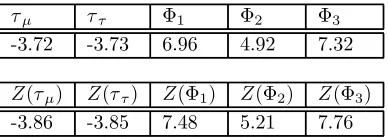
As a preliminary examination of the data, we tested for the presence of unit roots in the processes generating the time series, under the maintained hypothesis of linearity, using standard linear unit root tests, the results of which are reported in Table 1.18 In each case, consistent with the results of Lothian and Taylor
1 6For a full description of the earlier data and their sources see the appendix to Lothian and
Taylor (1996). While we have extended our data set from that used in Lothian and Taylor (1996) to include an additonal ten years or so of data up to 2001, we have had to discard some observations at the beginning of the sample because the population data we use begins only in 1820. Nevertheless, the data set still spans over 180 years.
1 7http://www.library.uu.nl/wesp/populstat/populhome.html.
1 8In particular, following Perron (1988) and Lothian and Taylor (1996), we estimated
equa-tions of the form:
qt=κ+λ(t−
T
2) +δqt−1+ut
whereT is the sample size andutis an error term. The following null hypotheses were then
tested:
HA:δ= 1; HB: (κ,λ,δ) = (0,0,1); HC: (λ,δ) = (0,1),
using either the standardt-statistics andF-statistics,ττ(although referred to the distributions
transforma-(1996) (although using data sampled over a slightly different period), we are able to reject the unit root hypothesis at the &ve percent level or lower.
We then proceeded to estimate linear autoregressive models for each of the real exchange rates, with a lag length of one year, as suggested by examination of the partial autocorrelation function for each of the series. The results are re-ported in Table 2 and they are qualitatively similar to those rere-ported by Lothian and Taylor (1996). Given the importance of data span in an analysis of low-frequency properties, it is perhaps not surprising, however, that the measured persistence of the two real exchange rates is slightly higher than that reported in our earlier work, where we used a slightly longer data set (1791-1990 for sterling dollar, as opposed to 1820-2001 in the present study, for example). Nevertheless, the point estimate of the autoregressive coefficient of0.902for sterling-dollar is close to the point estimate of0.887 of Lothian and Taylor (1996), and implies a half-life of adjustment of6.78years. Again in line with Lothian and Taylor (1996), the results for the sterling-franc imply a faster speed of adjustment, with a point estimate of the autoregressive coefficient of0.831 and a corresponding half-life estimate of3.75years.
In brief, therefore, the linear estimation results are noteworthy for two rea-sons, both of which serve to con&rm previous &ndings reported in the literature. First, it is possible to reject the unit root hypothesis at standard signi&cance levels using sufficiently long spans of data (Frankel, 1986; Lothian and Taylor, 1996, 1997). Second, although the unit root hypothesis can be rejected, the estimated half-lives of shocks to the real exchange rates involved are extremely slow ranging from about 3.75 to 6.78 years. Given that the volatility of real exchange rates implies that they must be largely driven by nominal and &nan-cial shocks which one would expect to mean revert at a much faster rate, this evidence is con&rmatory of Rogoffs purchasing power parity puzzle (Rogoff, 1996).
Note, however, that for sterling-franc there is signi&cant evidence of au-toregressive conditional heteroskedasticity (ARCH) in the estimated residuals. Although we have used heteroscedasticity-robust estimated standard errors, this does suggest that it may be fruitful to try and model this heteroscedasticity
di-tions of these statistics due to Phillips (1987) and Phillips and Perron (1988),Z(ττ),Z(Φ2) andZ(Φ3).
Phillips and Perron (1988) and Schwert (1989) demonstrate that the Phillips-Perron non-parametric test statistics may be subject to distortion in the presence of moving-average com-ponents in the time series. Accordingly, as in Lothian and Taylor (1996), we therefore tested for the presence of moving-average components and could detect no statistically signi&cant such effects in either of the real exchange rate series.
If the unit root hypothesis cannot be rejected at this stage, then greater test power may be obtained by estimating the equation:
qt=κ∗+δ∗qt−1+u∗t
and testing the hypotheses:
HD:δ∗= 1; HE: (κ∗,δ∗) = (0,1),
rectly. Alternatively or in addition the signi&cant ARCH test statistic may simply be indicative of signi&cant residual outliers, suggesting that the condi-tional mean is misspeci&ed in the linear formulation.
6.2
Nonlinear estimation results
6.2.1 univariate estimation results
Bringing together the previous discussion on modelling nonlinearity, the Harrod-Balassa-Samuelson effect and regime-varying volatility, we can now summarise our empirical nonlinear model. We treat the UK as the Home economy and, for notational convenience, we introduce a country subscript on parameters and variables. Thus,qF rance,tis the real exchange rate between the UK and France
andqU S,tis the real exchange rate between the UK and the US. Further, treating
the UK as the Home economy, Home productivity, denotedatin equation (12),
becomes UK productivity at timet, denotedaU K,t. The Foreign economy then
becomes either France or the US, so that the Foreign productivity variable of equation (12),a∗
t, becomes either French or US productivity, denoted aF rance,t
andaU S,t respectively. The full empirical model may thus be written, for i =
U S, F rance:
(qi,t−μi,t) =
Pp
j=1βi,j(qi,t−j−μi,t−j)
+hPpj=1β∗i,j(qi,t−j−μi,t−j)
i
×£1−exp[−θi(qi,t−d−μi,t−d)2]
¤
+εi,t (16)
μi,t =μi,0+μi,1aU K,t−μi,2ai,t (17)
εi,t∼N(0,σ2i,t) (18)
σ2i,t=σ2i,F loat[1−It{t∈F ix(i)}] +σ2i,F ixIt{t∈F ix(i)}. (19)
As before,It{.}is an indicator variable, equal to unity when the statement in
or from examination of the partial autocorrelation functions for the real ex-change rate adjusted for relative productivity.19 A &nal choice of &rst-order
autoregression thus imposes the restrictions βi,j = 0 and β∗i,j = 0, for j > 1. The delay parameter,d, was chosen using the procedure suggested by Granger and Teräsvirta (1993) and Teräsvirta (1994), as outlined in Section 2 and, as anticipated, a delay of one year appeared to capture adequately the nonlinear dynamics of the ESTAR transition function (d= 1).20 Further, the coefficient
on foreign productivity, when estimated freely, was numerically close to and insigni&cantly different from being equal to that on domestic productivity, so that productivity was entered in relative terms (μi,1 =μi,2). In addition, for both the US and France, the estimated value ofμi,0 was found to be insigni&-cantly different from zero at the &ve percent level and was set to zero (μi,0= 0). Finally, unrestricted estimates ofβi,1andβ∗i,1were numerically close to plus and minus unity, respectively, and the restrictionsβi,1= 1andβ∗i,1=−1could not be rejected at the &ve percent level and were imposed.
Substituting (17) into (16), imposing these restrictions and rearranging, our &nal parsimonious empirical speci&cations were therefore of the form:21
[qi,t−μi,1(aU K,t−ai,t)] = [qi,t−1−μi,1(aU K,t−1−ai,t−1)] (20)
×exp£−θi[qi,t−1−μi,1(aU K,t−1−ai,t−1)]2¤+εi,t
εi,t∼N(0,σ2i,t) (21)
σ2i,t=σ2i,F loat[1−It{t∈F ix(i)}] +σ2i,F ixIt{t∈F ix(i)}. (22)
1 9As noted in Section 2, Granger and Teräsvirta (1993) suggest determining the order of
the autoregression in STAR models by examination of the partial autocorrelation function (PACF). This is problematic in the present case, however, since we are jointly estimating the time-varying mean of the series to which we are simultaneously &tting an ESTAR model i.e.(qi,t−μi,t)≡[qi,t−(μi,0+μi,1aU K,t−μi,2ai,t)].While examination of the PACF for
each of the real exchange rates and each of the productivity series did indeed suggest nothing greater than &rst-order serial correlation, it is well known that a linear combination of AR(1) processes may not necessarily be AR(1) (Granger and Morris, 1976). However, the PACF for the real exchange rate series adjusted for relative productivity, i.e. [qi,t−(aU K,t−ai,t)], also
appeared to be exhibit at most &rst-order serial correlation and, together with our intuitive preference for &rst-order model with annual data, it therefore seemed reasonable to proceed on this basis. We did, however, check for remaining serial correlation in the &nal estimated models (and found none).
2 0In addition, terms involving third-order powers of y
t−dwere in every case insigni&cant
in the estimated auxiliary regressions, implying that a logistic transition function could be rejected in favour of an exponential transition function.
2 1Note that the transition function in (20) is of the form exp[.]rather than the standard
ESTAR transition function of the form{1−exp[.]}, as in (16). This is because, with a &rst-order autoregression (βi,j = 0and β∗i,j = 0, for j > 1), the further restrictions βi,1 = 1 and β∗
i,1 = −1 imply that deviations from long-run equilibrium follow a random walk in the close neighbourhood of equilibrium, whenexp£−θi[qi,t−1−μi,1(aU K,t−1−ai,t−1)]2¤≈ exp [0] = 1, but become increasingly mean-reverting as the size of the deviation grows and
exp£−θi[qi,t−1−μi,1(aU K,t−1−ai,t−1)]2 ¤
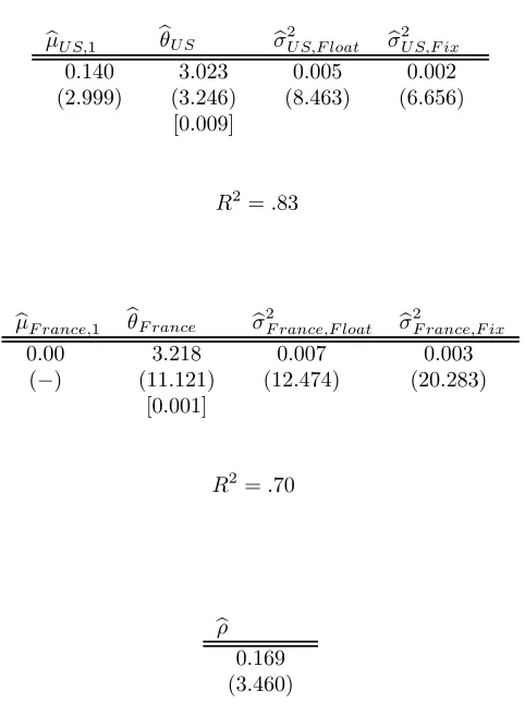
The univariate estimation results of this model, obtained by maximum like-lihood estimation, are reported in Table 3. In both cases, a good &t is indicated, with the coefficient of determination in each case improving upon that obtained using a linear model (compare Table 2). Moreover, the residual diagnostics (calculated using the residuals standardized by the square root of the estimated variance function) are in each case satisfactory.22 The major difference between
the US and French results is that, for sterling-franc, the estimated coefficient
b
μF rance,1 was found to be insigni&cant at the &ve percent level and was set to
zero.
These estimation results are noteworthy for a number of reasons. First, there is signi&cant evidence of nonlinear mean reversion, as shown by the fact that the estimated transition parameterbθiis in both cases strongly signi&cantly
different from zero. Note, however, that the ratio of this estimated coefficient to its standard error the t-ratio cannot be referred to the Student-t or normal distribution for purposes of inference, since under the null hypothesis H0:θi= 0,qi,tfollows a linear unit root process.23 This introduces a singularity
under the null hypothesis so that standard inference procedures cannot be used, analogously to the way in which standard inference procedures cannot be used in the usual Dickey-Fuller or augmented Dickey-Fuller tests for a linear unit root. Indeed, testing the null hypothesisH0:θi= 0is tantamount to a test of the null
hypothesis against the alternative hypothesis of nonlinear mean reversion, rather than against the alternative of linear mean reversion.24 Therefore, because the
distribution of the estimator of θi is unknown under the null hypothesis, we
calculated the empirical marginal signi&cance level of the ratio of the estimated coefficient to the estimated standard error by Monte Carlo methods under the null hypothesis that the true data generating process for the logarithm of both of the real exchange rate series was a random walk, with the parameters of the data generating process calibrated using the actual real exchange rate data over the sample period.25 From these empirical marginal signi&cance levels (reported in square brackets below the coefficient estimates in Table 3), we see that the estimated transition parameter is signi&cantly different from zero with a marginal signi&cance level of virtually zero in each case. Since these tests may
2 2Note that these residual diagnostics should be treated only as indicative, since the
stan-dardized residuals are functions of estimated variance parameters.
2 3In addition, under the null hypothesis,H
0:θi= 0, the autoregressive parameters of the
nonlinear part of the speci&cation are unidenti&ed see Davies (1987), Hansen (1996).
2 4Our approach may thus be seen in some ways to be equivalent to unit root tests with
the alternative of smooth transiton nonlinearity as developed by Kapetenios, Shin and Snell (2003). Eklund (2003) develops a joint test of nonstationarity and linearity &nds that the linear unit root hypothesis can be rejected in favour of nonlinear mean reversion for a number of real exchange rates, consistent with the approach in this paper and in Taylor, Peel and Sarno (2001).
2 5The empirical signi&cance levels were based on5,000simulations of length280, initialized
be construed as nonlinear unit root tests, the results indicate strong evidence of nonlinear mean reversion for each of the real exchange rates examined over the sample period.
Second, the estimated coefficient for the relative productivity term, bμi,1 is strongly signi&cantly different from zero for the case of sterling-dollar (an asymp-totic t-ratio of nearly eight) and is correctly signed according to the Harrod-Balassa-Samuelson effect: relatively higher US productivity generates a real ap-preciation of the equilibrium value of the dollar against the pound. For the case of sterling-franc, however, there is no signi&cant evidence of the HBS effect.26
6.2.2 joint estimation results
In order to gain efficiency in the estimation, we also estimated the US and French equations jointly by full information maximum likelihood (FIML), assuming a constant correlation coefficient between the French and US regression errors, so that the covariance matrix takes the form:
∙
εU S,t
εF rance,t
¸
∼N(O,Σt) (23)
Σt= ∙
σ2
U S,t ρ·σU S,t·σF rance,t
ρ·σU S,t·σF rance,t σ2F rance,t
¸
(24)
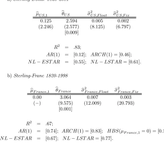
whereσ2i,t(i=U S, F rance) is as de&ned in (15) andρis the constant correla-tion coefficient. The joint estimation results are reported in Table 4.27
The FIML estimates of the residual variances are almost identical to those obtained using single-equation maximum likelihood, and the estimated correla-tion coefficient between the US and French residual series is strongly signi&cantly different from zero, with a point estimate of0.169. Moreover, the HBS slope coefficient is again signi&cantly different from zero at the &ve percent level only for the US, for which there is a slight increase in the point estimate of this coefficient from 0.125 to 0.140. Perhaps the most striking aspect of the FIML estimation results, however, is the increase in the point estimates of the tran-sition parameter,bθi, which increases from2.594 to 3.023 for the US and from
3.064to3.218for France. We again calculated the empirical distribution of the t−ratios for the estimated transition parameters, and they were each found to be highly signi&cantly different from zero.28
2 6These results are in line with the present authors conjecture in Lothian and Taylor (2000),
based on an analysis of nonlinear trends in these real exchange rates.
2 7Since the franc ceased to exist after 1998, the joint estimation results are for the sample
period 1820-1998.
2 8The empirical distributions of the t−ratios forθ
iwere calculated similarly to the
univari-ate case as described above (i.e. from Monte Carlo experiments in which the data generating process is a random walk), except that they were based on joint estimation of the French and US models.
6.2.3 calculating the average speed of mean reversion
We proceeded to gain a measure of the mean-reverting properties of the esti-mated nonlinear models through calculation of their implied half-lives, using the models estimated by FIML.29 Effectively, this involves comparing the
impulse-response functions of the models with and without initial shocks. Thus, we examined the dynamic adjustment in response to shocks through impulse re-sponse functions which record the expected effect of a shock at time t on the system at timet+j. For a univariate linear model, the impulse response function is equivalent to a plot of the coefficients of the moving average representation (see e.g. Hamilton, 1994, p. 318). Estimating the impulse response function for a nonlinear model, however, raises special problems both of interpretation and of computation (Gallant, Rossi and Tauchen, 1993; Koop, Pesaran and Potter, 1996). In particular, with nonlinear models, the shape of the impulse-response function is not independent with respect to either the history of the system at the time the shock occurs, the size of the shock considered, or the distribution of future exogenous innovations. Exact estimates can only be produced for a given shock size and initial condition by multiple integration of the nonlinear function with respect to the distribution function each of the j future inno-vations, which is computationally impracticable for the long forecast horizons required in impulse response analysis.
In the research reported in this paper, we calculated the impulse response functions, both conditional on average initial history and conditional on initial real exchange rate equilibrium, using the Monte Carlo integration method dis-cussed by Gallant, Rossi and Tauchen (1993). The basic idea is to calculate a baseline forecast for a large number of periods ahead using the estimated model. We then calculate a second forecast but this time with a shock in the initial pe-riod. The difference between the baseline forecast path and the shocked forecast path then gives the impulse response function. In each case, the forecast path is calculated by simulating the model a large number of times and taking the average. The discrete number of years it takes for the effect of the shock on the level of the real exchange rate to dissipate by &fty percent is then taken as the estimated half life for that size of shock.30
We carried out two sets of simulations, one in which the real exchange rate is assumed to be at its long-run equilibrium prior to the shock, and one in which the real exchange rate response is calculated taking the average value of the real exchange rate over the Bretton Woods period as the initial value.31
2 9Using the models estimated by univariate maximum likelihood resulted in qualitatively
identical results.
3 0This de&nition of the half-life may be problematic where the impulse response function is
non-monotonic, since the effect of the shock on the level of the real exchange rate may drop below &fty percent of its initial value and then rise above it again. Fortunately, in the cases examined in this paper, this was not the case.
3 1All simulations were carried out using initial values of the variables corresponding to
The estimated half-lives of the two real exchange rate models, calculated for six sizes of shock, conditional on average initial history over the post-Bretton woods sample periods period (1973−2001 for sterling-dollar, 1973−1998for sterling-franc), or on initial equilibrium, are shown in Table 5.32 They illustrate
well the nonlinear nature of the estimated real exchange rate models, with larger shocks mean reverting much faster than smaller shocks and shocks conditional on average history mean reverting much faster than those conditional on initial equilibrium. In particular, for shocks of ten percent or less and conditional on average initial history, the half-life is in both cases two years, while larger shocks
b
μi,1(aU K,t−1−ai,t−1)fori=U S, F rance, wherebμi,1denotes the values reported in Table 4, i.e.μbU S,1= 0.140andbμF rance,1= 0. We then used a total of5,000replications to produce each next-step-ahead forecast in the sequence, conditional on the previous forecast, and took the average over the5,000as the forecast value for that step. This is done for20steps ahead, with and without an additive shock at time tand the sequence representing the difference between the two paths is taken as the impulse response function. Since we use a large number of simulations, by the Law of Large Numbers this procedure should produce results virtually identical to that which would result from calculating the exact response functions analytically by multiple integration (Gallant, Rossi and Tauchen, 1993).
This procedure was then modi&ed as follows in order to produce an estimate of the impulse-response function conditional on the average history of each of the real exchange rates. Starting at the &rst data point (for 1974), qi,t−1 is set equal to {|qi,1973− b
μi,1(aU K,1973−ai,1973)|+μbi,1(aU K,1973−ai,1973)}. If[qi,1973−bμi,1(aU K,1973−ai,1973)]>0, this is just qi,1973 itself. If, however, [qi,1973−bμi,1(aU K,1973 −ai,1973)] < 0, then {|qi,1973−μbi,1(aU K,1973−ai,1973)|+bμi,1(aU K,1973−ai,1973)} is the number which is an equal absolute distance above the estimated equilibrium value bμi,1(aU K,1973−ai,1973) as qi,1973is below it. This transformation is necessary because we consider only positive shocks and it is innocuous because of the symmetric nature of ESTAR adjustment below and above equilibrium. A20-step forecast is then produced using200 replications at each step, with and without a positive shock of sizelog(1 +k/100) at timet, using the estimated ESTAR model, and realizations of the differences between the two forecasts are calculated and stored as before. We then move up one data point (hence settingt−1 = 1974), and repeat this procedure. Once this has been done for every data point up to the end of the sample period, an average over all of the simulated sequences of differences in the paths of the real exchange rates with and without the shock at timetis taken as the estimated impulse response function conditional on the average history of the given exchange rate and for a given shock size.
3 2For linear time series models the size of shock used to trace out an impulse response
function is not of particular interest since it serves only as a scale factor, but it is of crucial importance in the nonlinear case. In the present application we are particularly concerned with the effect of shocks to the level of the real exchange rate. Given a particular value of the log real exchange rate at time t, qi,t whether this be the historical value or the
estimated equilibrium level a shock of k percent to the level of the real exchange rate involves augmentingqi,tadditively bylog(1 +k/100). (For smallk,log(1 +k/100)is of course
approximately equal tok/100. This approximation is not, however, good for the larger shocks considered in this paper.) This raises a problem, however, in the calculation of the half-lives, since although the natural measure might be the discrete number of years taken until the shock to the level of the real exchange rate has dissipated by a half i.e. when the impulse response function falls belowlog(1 +k/200) this would make comparisons with previous research on linear time series models of real exchange rates difficult. Accordingly, although we de&ne ak percent shock to the real rate as equivalent to addinglog(1 +k/100)toqi,t, we calculate the
half life as the discrete number of years taken for the impulse response function to fall below
have a half life of one year or less. These results therefore accord broadly with those reported in Taylor et al. (2001), and shed some light on Rogoffs (1996) PPP puzzle . Only for small shocks occurring when the real exchange rate is near its equilibrium do our nonlinear models consistently yield very long half lives in the range of three to &ve years or more, which Rogoff (1996) terms glacial . Once nonlinearity is allowed for, even small shocks of one to &ve percent have a half life of two years or less, conditional on average history, and for larger shocks the speed of mean reversion is even faster.33
6.3
How important is the Harrod-Balassa-Samuelson
Ef-fect?
In Figure 1 we have plotted the sterling-dollar real exchange rate together with our measure of the Harrod-Balassa-Samuelson term, HBSt = bμU S,1(aU K,t−
aU S,t), where bμU S,1is the &tted value of μU S,1 from Table 4. It is interesting
how relative productivity captures the underlying trend depreciation of the real value of sterling against the dollar over this very long period. On the other hand, this raises the question of whether this common trend is purely a statis-tical artefact rather than an economic relationship. Our nonlinear estimation results do indicate that the Harrod-Balassa-Samuelson effect is strongly statisti-cally signi&cant in explaining movements in the equilibrium real exchange rate for sterling-dollar but not for sterling-franc over the one-hundred-and-eighty-year period under investigation. However, statistical signi&cance is not quite the same thing as economic signi&cance. In particular, if the Harrod-Balassa-Samuelson effect has been economically signi&cant, then it should de better at explaining real exchange rate movements than complex time trends and we should also perhaps expect it to account for a substantial proportion of the vari-ation in the real exchange rate over the sample period in question. Moreover, if reversion of the real exchaneg rate towards its fundamental equilibrium becomes stronger over longer time horizons, then the proportion of the variation in the real exchange rate explained by deviations from that equilibrium should be an increasing function of the time horizon. We investigated each of these issues.
6.3.1 trends, relative productivity and the real exchange rate
In Table 6, we report the results of some simple investigations of the impor-tance of the HBS effect for sterling-dollar. In panel a) we report the results of regressing the real exchange rate onto the relative productivity term alone,
(aU K,t−aU S,t). The estimated slope coefficient is highly signi&cant and the
R2 statistic reveals that the HBS effect appears to account for just over forty
percent of variation in the real exchange rate over the last one-hundred-and-eighty years. This accords with Rogoffs (1996) intuition that real exchange rate variation is driven largely by nominal shocks (some sixty percent on our
3 3The 95% con&dence bounds on the half lives were in every case less than one year in
measure) although a contribution of forty percent from the real side is clearly sizeable.
In panel b) of Table 5 we have reported the results of regressing relative productivity onto a cubic trend.34 In Lothian and Taylor (2000), we found that
a cubic trend was signi&cant when added to a real exchange rate autoregression for sterling-dollar, and we conjectured that this term was in fact proxying for HBS effects. The fact that the cubic trend is able to explain some 97 percent of the variation in the relative productivity term appears to con&rm this conjecture. In Lothian and Taylor (2000) we also pointed out, however, that a cubic trend in the HBS effect was to be expected on economic grounds also, given the increasing dominance of the UK over the US as an industrial power in the earlier part of the sample period, and the rise and subsequent dominance of the US over the UK in the later part of the sample period.
In panel c) of Table 5, we report the results of regressing the HBS-adjusted real exchange rate i.e.[qU S,t−bμU S,1(aU K,t−aU S,t)] onto its own lagged value
and the cubic trend terms. The cubic trend terms are found to be individually and jointly insigni&cantly different from zero, consistent with the results and conjectures of Lothian and Taylor (1997). In addition, note that, also consistent with the analysis and conjectures of Lothian and Taylor (2000), the estimated half life of adjustment drops dramatically in the HBS-adjusted autoregression, (from the estimate of 6.78 years reported for the unadjusted sterling-dollar real exchange rate in panel a) of Table 2) to 3.19 years. Although these results are clearly only indicative, especially given the importance we have demonstrated of allowing for nonlinear adjustment in real exchange rates, they are nevertheless striking.
6.3.2 explaining real exchange rate variation due to HBS effects at different time horizons
While the &nding that HBS effects accounted for about forty percent of real exchange rate variation for sterling-dollar over the whole sample period so that some sixty percent of the variation is due to nominal factors it seems likely that the contribution of real factors to real exchange rate movements will vary over different time horizons. In particular, it seems reasonable to expect nominal variablity to dominate mostly at shorter horizons, with real effects becoming more important at longer horizons.35 In order to investigate this possibility, we estimated long-horizon regressions of the form
(qU S,t+k−qU S,t) =α+γk[(aU K,t+k−aU S,t+k)−(aU K,t−aU S,t)] +νt (25)
whereαand γk are regression parameters, νt is the regression residual (which
will in general be serially correlated fork >1, since overlapping forecast errors
3 4The term cubic trend, is understood here to denote a function of time including terms in
tandt2as well ast3.
3 5Indeed, this seems to be the import of Rogoffs (1996) analysis of real exchange rate
will contain some common information). By regressing the change in the real exchange rate from periodtto periodt+konto the change in relative produc-tivity over the same period, this regression will capture the amount of variation in the k−year change in the real exchange rate that can be explained by the k−year change in the HBS effect.36 Thus, if nominal rather than real effects
dominate real exchange rate movements over short horizons, then we should expect a lowR2for regressions with low values ofkand increasing values of the R2 askincreases.
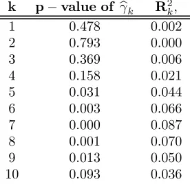
The results of estimating the long-horizon regression for values ofkfrom one to ten years are given in Table 7.37 They are in accordance with our intuition.
At the shortest horizon of one year, the change in productivity accounts for less than one percent of the variation in the annual change in the real exchange rate and the estimated value of γk has a p-value (marginal level of statistical signi&cance) of 0.47. It is not until the time horizon reaches &ve years that the estimated slope parameter becomes signi&cantly different from zero at the &ve percent level, with around four percent of the &ve-year real exchange rate change explained by the HBS effect. The signi&cance of the HBS effect reaches its peak at seven years, when nearly nine percent of the seven-year real exchange rate change is explained, after which it declines. By the tenth year, however, relative productivity is still signi&cant albeit at only the ten percent level in explaining the ten-year real exchange rate change, with around four percent explained.
7
Conclusion
A reading of the empirical literature on real exchange rates and purchasing power parity suggests a number of in! uences worthy of investigation. The &rst is the effect of real variables on the equilibrium levels of real exchange rates over the long run, and in particular the in! uence of relative productivity differentials the Harrod-Balassa-Samuelson effect. A second issue concerns the possibility of
3 6This is a variant on the standard long-horizon regression of the the k−period change of
a variable onto its deviation from equilibrium at timet. In the present context, the standard long-horizon regression would take the form
(qU S,t+k−qU S,t) =α+γk[qU S,t−bμU S,1(aU K,t−aU S,t)] +νt
A regression of this kind would be uninformative for our purposes, however, since the concept of real exchange rate equilibrium involves an element of pure PPP as well the HBS effect, and we wish to isolate the in! uence of the latter alone.
Long-horizon regressions have long been used in the &nance literature (see e.g. Campbell, Lo and MacKinlay, 1997). For applications to exchange rates, see Mark (1995), Chen and Mark (1996) and Kilian and Taylor (2003).
3 7It is well known that asymptotic critical values for the t-test statistics for the slope
nonlinear adjustment of real exchange rates to their long-run equilibria. A third relates to differences in real exchange rate volatility across nominal exchange rate regimes.
We have investigated all three sets of in! uences in the research reported in this paper. To do so, we have estimated exponential smooth transition autore-gressive (ESTAR) models for real sterling-dollar and real sterling-franc exchange rates in which we include relative real per capita income as a proxy for relative productivity and in which we allow for possible shifts in the variance of the errors. The data set that we use spans nearly two centuries and thereby allows not only enhanced test power but also provides an environment in which the various factors that in principle can affect real exchange-rate behaviour have sufficient scope to operate.
While we &nd evidence of signi&cant nonlinearities in adjustment for both exchange rates, we &nd signi&cant evidence of HBS effects for sterling-dollar but not for sterling-franc. There is also evidence of shifting real exchange rate volatility for both exchange rates, with higher volatility recorded during ! oating nominal exchange rate regimes.
We then go on to analyse the impulse-response functions for shocks of vary-ing magnitudes to the two real exchange rates. In both instances, these show greatly increased speeds of adjustment vis-à-vis those estimated with linear au-toregressive models for all but the very smallest shocks. Conditional on average initial history, the estimated half lives for large shocks of twenty per cent or more are only one year; for small shocks in the range of one to &ve percent they range from one to two years depending upon the exact magnitude of the shocks. While the HBS effect is able to explain some forty percent of the variation in the level of the sterling-dollar real exchange rate over the whole sample period, we found that the in! uence of real effects on the real exchange rate varies ac-cording to the time horizon considered. In particular, long-horizon regressions of thek−year change in the real exchange rate onto thek−year change in rela-tive productivity revelealed that at the shortest horizon of one year, HBS effects account for only a tiny proportion of the change in the real exchange rate. The proportion explained increases with the length of the time horizon, however, until it peaks at the seven-year horizon, when HBS effects explain around nine percent of the seven-year change in the real exchange rate.
This research might be fruitfully extended in a number of directions. First, investigation of the Harrod-Balassa-Samuelson effect in a nonlinear framework could be carried out for other countries, especially those that have experienced high rates of growth relative to the base country.38 Second, the analysis could
be repeated, focusing on the recent ! oating-rate period, and perhaps employ-ing nonlinear panel estimation methods for a group of countries. Third, the framework used in this paper could be extended to a multivariate nonlinear sys-tem involving nominal exchange rates and relative prices as well as productivity differentials, in order to examine the relative speed of adjustment of nominal ex-change rates and relative prices to deviations from the equilibrium real exex-change
rate.39
References
Asea, Patrick K, and Enrique Mendoza. 1994. The Balassa-Samuelson Model: A General Equilibrium Appraisal. Review of International Economics. 2, 244-67.
Balassa, Bela. 1964. The Purchasing-Power Parity Doctrine: A Reap-praisal. Journal of Political Economy. 72, pp. 584-96.
Baxter, Marianne., and Alan C. Stockman. 1989. Business Cycles and the Exchange Rate System. Journal of Monetary Economics 33, pp. 5-38.
Bergin, Paul R., Reuven Glick and Alan M. Taylor. 2004. Productivity, Tradability, and The Great Divergence. National Bureau of Economic Research Working Paper (June).
Campbell, John Y., Andrew W. Lo and A. Craig MacKinlay. 1997. The Econometrics of Financial Markets. Princeton, NJ: Princeton University Press. Cassel, Gustav. 1918. Abnormal Deviations in International Exchanges. Economic Journal 28, pp. 413-415.
Chen, Jian and Nelson C. Mark. 1996. Alternative Long-Horizon Exchange Rate Predictors International Journal of Finance and Economics, 1, pp. 229 250.
Cheung, Yin-Wong, Kon S. Lai and Michael Bergman. 2004 Dissecting the PPP Puzzle: The Unconventional Roles of Nominal Exchange Rate and Price Adjustments Journal of International Economics 64:1, pp. 135-50.
Chinn, Menzie D. 1999. On the Won and Other East Asian Currencies . International Journal of Finance and Economics 4:2, pp. 113-27.
Chinn, Menzie D., and Michael P. Dooley. 1999. International Monetary Arrangements in the Asia-Paci&c Before and After . Journal of Asian Eco-nomics, 10:3, pp. 361-84.
Clark, Gregory. 2001. The Secret History of the Industrial Revolution Unpublished working paper, Department of Economics, University of California at Davis.
Caner, Mehmet, and Lutz Kilian, 2001. Size Distortions of Tests of the Null Hypothesis of Stationarity: Evidence and Implications for the PPP Debate Journal of International Money and Finance 20, pp. 639-657.
Coakley, Jerry, Robert P. Flood, Ana-Maria Fuertes and Mark P. Taylor 2005 Purchasing Power Parity and the Theory of General Relativity: The First Tests Journal of International Money and Finance, 25, pp. 293-316.
Culver, Sarah E., and David H. Papell, 1999. Long-Run Purchasing Power Parity with Short-Run Data: Evidence with a Null Hypothesis of Stationarity Journal of International Money and Finance, 18, 751-68.
Davies, R.B. 1987. Hypothesis Testing When a Nuisance Parameter is Present Only Under the Alternative. Biometrika 74, pp. 33-43.
Dickey, David A., and Wayne A. Fuller. 1981. Likelihood Ratio Statisitcs for Autoregressive Time Series with a Unit Root. Journal of the American Statistical Association 74, p. 427-31.
Eichengreen, Barry. 1988. Real Exchange Rate Behavior Under Alterna-tive International Monetary Regimes: Interwar Evidence. European Economic Review. 32, pp. 363-71.
Eitrheim, Oyvind, and Timo Terasvirta. 1996. Testing the Adequacy of Smooth Transition Autoregressive Models. Journal of Econometrics 74:11, pp. 59-75.
Eklund, Bruno. 2003. A Nonlinear Alternative to the Unit Root Hy-pothesis SSE/EFI Working Paper Series in Economics and Finance, No. 547, Stockholm School of Economics.
Engel, Charles. 1999. Accounting for U.S. Real Exchange Rate Changes. Journal of Political Economy. 107:3, pp. 507-38.
Engel, Charles. 2000. Long-Run PPP May Not Hold After All. Journal of International Economics. 51, pp. 243-73.
Engel, Charles, and Chang-Jin Kim. 1999. The Long-Run U.S./U.K. Real Exchange Rate. Journal of Money, Credit and Banking, 31, pp. 335-55.
Engle, Robert and Clive W. J. Granger. 1987. Co-integration and Error Correction: Representation, Estimation and Testing. Econometrica. 55:2, pp. 251-76.
Feinstein, Charles H. 1972. National Income, Expenditure and Output of the United Kingdom, 1856-1965. Cambridge: Cambridge University Press.
Fisher, Eric O N, and Joon Y. Park 1991 Testing Purchasing Power Parity under the Null Hypothesis of Co-integration Economic Journal, 101, 1476-84. Flood, Robert P. and Andrew K. Rose. 1995. Fixing Exchange Rates: A Virtual Quest for Fundamentals. Journal of Monetary Economics. 36:1, pp. 3-37.
Flood, Robert P. and Mark P. Taylor. 1996. Exchange Rate Economics: What s Wrong with the Conventional Macro Approach?, in Jeffrey A. Frankel, Giovanni Galli and Alberto Giovannini (eds.), The Microstructure of Foreign Exchange Markets. Chicago: Chicago University Press.
Frankel, Jeffrey A. 1986. International Capital Mobility and Crowding-out in the U.S. Economy: Imperfect Integration of Financial Markets or of Goods Markets?, in How Open is the U.S. Economy? R. W. Hafer ed. Lexington, Mass.: Lexington Books, pp. 33-67.
Frankel, Jeffrey A. and Andrew K. Rose. 1995. Empirical research on Nominal Exchange Rates, in Handbook of International Economics, Volume 3. G. Grossman and K. Rogoff, eds. Amsterdam, New York and Oxford: Elsevier, North-Holland.
Frankel, Jeffrey A. and Andrew K. Rose. 1996. A Panel Project on Pur-chasing Power Parity: Mean Reversion Within and Between Countries. Journal of International Economics. 40:1-2, pp. 209-24.
Froot, Kenneth A. and Kenneth Rogoff. 1991. The EMS, the EMU, and the Transition to a Common Currency , in Stanley Fischer and Olivier Blan-chard (eds.) National Bureau of Economic Research Macroeconomics Annual. Cambridge, MA: MIT Press.
Grossman and K. Rogoff, eds. Amsterdam: North Holland, pp. 1647-88. Fuller, Wayne A. 1976. Introduction to Statistical Time Series. New York: John Wiley.
Gallant, A. Ronald, Peter E. Rossi, and George Tauchen. 1993. Nonlinear Dynamic Structures. Econometrica 61:4, pp. 871-907.
Granger, Clive W. J., and Michael J. Morris. 1976. Time Series Mod-elling and Interpretation Journal of the Royal Statistical Society, Series A.,139, pp.246-257.
Granger, Clive W. J. and Timo Teräsvirta. 1993. Modelling Nonlinear Economic Relationships. Oxford: Oxford University Press.
Hamilton, James D. 1994. Time Series Analysis. Princeton: Princeton University Press.
Hansen, Bruce E. 1996. Inference when a Nuisance Parameter is Not Iden-ti&ed under the Null Hypothesis. Econometrica 64, pp. 413-30.
Harrod, Roy. 1933. International Economics. London: Nisbet and Cam-bridge University Press.
Imbs, Jean, Haroon Mumtaz, Morten O. Ravn and Hélène Rey, 2003. Non-Linearities and Real Exchange Rate Dynamics. Journal of the European Eco-nomic Association , 1:2-3, pp. 639-649.
Imbs, Jean, Haroon Mumtaz, Morten O. Ravn and Hélène Rey, 2005. PPP Strikes Back: Aggregation and the Real Exchange Rate. Quarterly Journal of Economics, 120:1, pp.1-43.
Kapetanios, George, Yongcheol Shin and Andy Snell, 2003. Testing for a Unit Root in the Nonlinear STAR Framework Journal of Econometrics, 112, pp. 359-379.
Kilian, Lutz and Mark P. Taylor. 2003. Why Is It So Difficult to Beat the Random Walk Forecast of Exchange Rates? Journal of International Eco-nomics. 60:1, pp. 85-107.
Koop, Gary, M. Hashem Pesaran, and Simon M. Potter. 1996. Impulse Response Analysis in Nonlinear Multivariate Models. Journal of Econometrics 74:1, pp. 1-32
Lothian, James R. 1990. A Century Plus of Japanese Exchange Rate Be-havior. Japan and the World Economy. 2, pp. 47-50.
Lothian, James R. 1991. A History of Yen Exchange Rates, in W.T Ziemba, W. Bailey and Y. Hamao (eds.), Japanese Financial Market Research, Amsterdam: Elsevier.
Lothian, James R. 1997. Multi-country Evidence on the Behavior of Pur-chasing Power Parity under the Current Float. Journal of International Money and Finance 16, pp. 19-35.
Lothian, James R. and Mark P. Taylor. 1996. Real Exchange Rate Be-havior: The Recent Float From the Perspective of the Past Two Centuries. Journal of Political Economy. 104:3, pp. 488-509.