Comparison of iterative eigenvalue solvers for photonic crystal modeling

(1)

UNIVERSITY OF TWENTE

Comparison Of Iterative

Eigenvalue Solvers For

Photonic Crystal Modeling

Bachelor Assignment

Chairperson: Prof.Dr.Ir. J.J.W. van der Vegt

Daily supervisor: Dr. M.A. Bochev External Member: Prof.Dr.Ir. A. de Boer

Jelmer Gietema - s1065211

6/24/2014

This report describes of the eigenvalue computation in photonic crystal modeling of common two and three dimensional structures. A comparison between a number of solvers, parameters, and

(2)

2

1. Photonic Crystals

Crystals are constructed by a periodic arrangement of identical structural units in space which occurs in nature for example at atoms or molecules, but also at larger scale. The pattern with which the atoms, molecules or elements are repeated in space is the crystal lattice [1]. A Photonic Crystal (PC) has a surprising structure whit such a repeated construction of different layers. At a PC these layers differ in dielectric permittivity, i.e. in the ability to store electrical energy in an electric field. Due to differences in energy storage the refraction indices of the layers are influenced, by this each layer can have a different refraction index [2]. Also the geometry of the lattice dictates the conduction

properties of the crystal. PCs can be formed in different dimensions, whereas the simplest form is the one dimensional (1D) form. This 1D PC consists of alternating layers of material with different

dielectric constants; this is called a multilayer film. A more complex system is the two dimensional (2D) form. This crystal is periodic along two axes and homogeneous along the third axis. The most complex system is the three dimensional (3D) form. An overview of these three different types of PCS is given in figure one [1].

The length scale, for every direction, in which the variation takes place, determines the spectral range of functioning of the PC, and the wavelength at which the effects are felt. PCs working in the optical range of the electromagnetic (EM) spectrum will present a modulation of the dielectric function with a period of order of one micrometer. These structures present iridescences as a result of diffraction. This occurs also in nature, e.g. in a wing of a butterfly [3]. Depending on the shapes and permittivities of the dielectric materials, PCs produce so called band gaps for various frequency regions. PCs with specific band structures are of practical interest and have been extensively studied over the past few decades [1,2].

(5)

5

1.1 Band Gap

Photonic band gaps occur in the plane of periodicity, for the 1D structure this is in the x direction, for the 2D structure this is in the x-, and y direction, and for the 3D structure in x-, y-, and z direction [1]. A band gap, also called an energy gap, can be seen as a range in a solid where no electron states can exist, i.e. the propagation of electromagnetic waves is prohibited for all wave vectors. Due to this gap the wave equation will have different energy levels. The higher frequency modes store their energy in the lower permittivity layers, whereas the lower frequency modes store their energy in the layers with higher permittivity value [1]. The band gap occurs due to the differences in permittivity of the layers. The difference between those layers, i.e. the size of the gap, depends on the dielectric contrast. How bigger the contrast, the wider the gap. Band gaps in the energy band structure of the crystal means that electrons are forbidden to propagate with certain energies in certain directions, i.e. no radiation is expected from the dipole [3]. By use of this, one can steer the wave at certain frequencies. If the lattice potential is strong enough, the gap can extend to cover all possible propagation directions, resulting in a complete band gap. This means no electrons are allowed to move at this state, and incident light is reflected [1].

The bands above and below the gap can be distinguished by where the energy of their mode is concentrated. The low permittivity layers are for example air regions, which are above the band gap, and the high permittivity layers are the dielectric regions, which are below the band gap [1]. An overview can be found in figure 2.

Figure 2: Photonic Band structure of a multilayer film (1D). The width of the

layer is 0.3, and the width of the layer is 0.8a. [1]

(6)

6 Figure 3: The two dimensional structure of a Photonic Crystal [1]

For a PC of the 2D form a photonic band gap can occur in the xy plane. Such a 2D PC can prevent light from propagating in any direction within the plane. Due to the system being homogeneous in the z direction, the system has modes which must be oscillatory in this direction, with no restrictions on the wave vector. Any modes that propagate strictly parallel to the xy plane are invariant under reflections through the xy plane. The mirror symmetry allows us to classify the modes by separating them into two distinct polarizations, transverse electric (TE) and transverse magnetic (TM). Both can have different band structures [1].

PC structures can be built in different ways, how they are built depends on the purpose of the structure. One can add certain defects in this structure to trap modes or steer light. The simplest defect is a point defect, by this a single or multiple column(s) need(s) to be removed or replaced by a different dielectric material. Hereby we create a single localized mode or a set of closely spaced modes that have frequencies within the gap. The mirror symmetry is still intact. This defect may cause a peak into the crystal’s density of states (DOS), i.e. a peak in number of available states in the system, within the photonic band gap [1]. If so, the defect-induced state must be evanescent. The mode cannot penetrate into the rest of the crystal, since it has a frequency in the band gap. By removing a rod from the lattice structure we create a cavity that is effectively surrounded by

(7)

7

1.2 Applications

The function of the band gap in PCs can be used in many applications. Applications of PCs can be divided according to their principle of functioning. Some rely on the existence or non-existence of a complete gap, other rely on the peculiar properties of the bands and their dispersion. Applications that rely on a gap make use of the suppressed DOS, e.g. solar cells. If absorption can be neglected (thin structures) such an unusually large band gap can be used to recycle infrared blackbody

radiation into the visible spectrum. By this energy is not wasted in heat generation, but channeled by a thermal equilibrium into useful emission at the edge of the band gap [3].

Spontaneous emission is not inherent to an emitter, but rather depends on its electromagnetic environment. In a microcavity, the spontaneous emission rate can be greatly enhanced compared with that in free space. This so-called Purcell effect can dramatically increase laser modulation speeds [6]. A laser is a device that generates an intense beam of coherent monochromatic light (or other electromagnetic radiation) by stimulated emission of photons from excited atoms or

molecules. Spontaneous emission is the main foe to gain excited atoms as it happens isotropically and cannot be prevented by cavities. Cavities with a 3D complete gap present advantages in the sense that a single channel may be allowed for emission blocking other directions at the same time. Cavities in 2D systems are expected to present quality factors as high as tens of thousands and have already been realized with several thousands. Nowadays, research groups like LPNO and COPS are studying on the effects of photonic crystals on lasers to maintain the steady development to even faster and smaller devices, like mobile phones [3].

Also by propagation being normal to the equi-energy surfaces, i.e. the kinetic energy is the same for each degree of freedom in this system in thermal equilibrium, slight changes in wave vectors cause a strong bending of the beam. Similarly, if bending changes sign, ample changes in wave vector

(8)

8 Figure 4: PC can create a strong chromatic separation (a) in comparison with almost no separation

at a conventional crystal (b). This separation effect is called a superprism effect [3]

Another important application is slowing light down for example by use of chips and computers. This can already be done with a 2D PC structure with a point defect. Such a channel guide can easily present a region of frequencies in which guided waves have very low group velocities. The dispersion curves of the guided modes within the photonic band gap can be modified by altering the properties of the PC [9].

1.3 Eigenvalues

The eigenvalues can tell us a lot about the whole system. They describe the linear transformations. The eigenvectors can be seen as the axes along which a linear transformation acts simply by

stretching/compressing and/or flipping; eigenvalues give you the factors by which this compression occurs. By having more eigenvalues one knows more about the directions along the transformations occur and thus can understand more easily how the linear transformation acts. In fact, one tries to simplify the problem by use of eigenvalues and in that way has to solve an easier problem, with for instance fewer variables.

(9)

9

2. Maxwell’s Equations and

Frequency Domain Modeling

To find the frequency bounds without use of matrix multiplications we use eigenvalues. These eigenvalues can be derived from the Maxwell Equations. These four equations describe how

magnetic and electric fields are generated and altered by each other and by charges and currents. By this we can describe the electromagnetic states of the PCs.

2.1 Maxwell’s Equations

The Maxwell equations are, at the length scales of photonic crystals, for macroscopic view practically exact. The equations in three dimensions and with source currents are stated as

Here is the vector that denotes the position and denotes the time. is the electric current density and is the nonphysical magnetic current density. , and are the electric and magnetic field respectively and , and are the magnetic induction field and the electric displacement current.

By use of [1] we apply the constitutive relationships

Here is the relative permittivity and is the vacuum permittivity. is the relative permeability and is the vacuum permeability.

The electric current density consists of two components: the electric losses are of the form and a independent source term given by . Also for the magnetic losses we have two components: the magnetic losses and the independent source .

If we implement these functions in the stated Maxwell Equations we get

(10)

10

2.2 Second Order Differential Equation for

By use of the above four given equations of Maxwell we are able to derive one equation for , this will later on be derived for strictly the z direction.

By this we have a function for , we also know what is equal to

If we fill this into the equation we obtain one second order equation for .

In this situation we have the magnetic and electric current source, present in the right hand side. By this we have derived the equation for in 3D, but we need it to know for the z direction. This leads to

(11)

11

This results in

2.3 TM

z

_Mode

TMz stands for the transverse magnetic mode in the z direction. This indicates that the magnetic field is perpendicular to the z axis.

By use of [11] we can state the following relations

For a check if the function in the previous chapter is right we use the functions given above. We derive this in the same way as we derived the function for 3D. After the calculations are done we got the same function, thus this is correct.

2.4 Conditions

We now have a formula with a lot of variables, where some of them are equal to zero or set to zero, this all due to the artificial absorbing boundary conditions, the periodic conditions, and the Dirichlet condition. By this we have

(12)

12 Filling out these conditions results in the next equation

The equation above could be derived in two ways. At first we could have used the 2D TMz mode, i.e.

and after this the derivation of the second order equation for . Or we could have first derived this second order equation for and then go to 2D, i.e. .

2.5 Dimensionless form

For practical use we transform the equations, given with their real physical units, to scales of electric and magnetic field in such a way that the difference in magnitude is eliminated and all variables are rendered dimensionless.

First we introduce two scalar parameters: the typical length L in meters and the typical magnetic strength in . Thereby we use that equals , which is the impedance of vacuum, and we use

as the speed of light in a vacuum equally to .

From now on we will denote all variables with SI units with a subscript ‘ ’ and the resulting dimensionless variables without a subscript. Implementing the subscript

We will transform our variables with the following transformations as defined above. By use of [11] we can state

Once implemented, and with use of the relation between and this will result in

For a frequency in SI units we get the following relation

(13)

13

2.6 Frequency domain

We suppose is of the form

This can be stated due to being a wave, i.e. this is in the most cases true and thus a reliable assumption. If we implement this in the derived equation we finally end up with

2.7 Discretization

We need to derive this function by use of Matlab; therefore we need to discretizise the function. This is done by dividing the length of x in k pieces which are evenly distributed, the same yields for y which is divided in j pieces. Thus we have:

If we fill this out for the electric field we get

The equation is a second order differential equation to both x- and y directions. This can be

calculated by use of the Finite Difference method. Here one makes use of nodes; one calculates the certain value at every node and this will finally end up in the total equation. By use of [19, pp 62-65] we can derive the following equations for the derivatives of . By this in combination with the discretization we can write

as

Any terms that refer to nodes on the boundary are set to zero, due to PEC boundary conditions.

2.8 Eigenvalue Problem

The equation stated above can be written as the generalized eigenvalue problem (GEP).

with

(14)

14

Here is the so called eigenvalue for this system and is the so called eigenvector. The

eigenvector is in this case the electric magnetic field in the z direction. The matrix is the double curl operator and it is Hermitian and positive semi-definite. is a positive and diagonal matrix. The matrix influences the spectrum of the GEP and thus the band structure of the corresponding PC [2]. The matrices are influenced by the dielectric materials in the PCs, which influences the band gap. Thereby the band gap is of very importance for the PC and its applications as stated before.

The difficulty of solving this equation depends on the structure of the PC. The matrix is a double curl operator which in simple cubic conditions is considered easier to solve due to they are mutually independent due to the pair wise orthogonal simple cubic lattice vectors. By this standard Fast Fourier Transform (FFT) can be applied to solve the corresponding eigenvalue problems. Eigenvectors associated with the FCC lattice are mutually dependent, due to the pair wise non-orthogonal FCC lattice vectors. Here standard FFT techniques cannot be applied to these periodic coupling

(15)

15

3. Eigenproblem Solvers

3.1 Methods

3.1.1 Generalized Eigenvalue Problem (GEP)

The GEP can be solved by use of different methods, i.e. different solvers. One such a method is solving the problem in the direct way. This can be done by the Eigs function of Matlab. Eigs uses the Arnoldi or the Lanczos basis to solve the Krylov space of the problem

.

The Krylov basis is defined in [14,15]. For our problem the overall function, used for Eigs in Matlab is >> Eigenvalues = eigs(A,B,6,50,opts);

The parameters are discussed later on.

Another method is to solve this problem by use of an iterative solver, such as the Jacobi-Davidson (JD) solver. By use of an iterative solver one can use a preconditioner to improve the performance of the solver, if chosen right. The JD can also be used without preconditioner to solve the problem

_. Where

is called the projection. Sigma can vary a little. For our problem the overall function used for JD in Matlab is

>> [V,D,flag] = jdqr('matvec_BinvA',N,K,sigma,param_jdqr); The parameters are discussed later on.

3.1.2 Null Space Free Eigenvalue Problem (NFEP)

The matrices in our problem consist of lots of zero’s. If we need to get rid of this issue of the null space one can transform the GEP into a NFEP. By this the hard problem of finding the smallest positive eigenvalues that are of interest is tackled. After some calculations the GEP will results in

where

(16)

16

and

Here is the coefficient matrix. is the diagonal matrix containing the elements of material dependent dielectric constants, is a positive diagonal matrix, and is an orthogonal basis.

are the diagonal matrices, corresponds to the regular finite difference, and is a unitary matrix. More detail on this transformation can be found in [4].

The approach of transforming GEP to NFEP is designed for finite difference discretizations. Which is not the case for our problem.

3.1.2.1 Shift-Invert Residual Arnoldi method for NFEP

The Shift-Invert Residual Arnoldi method (SIRA) solves the standard eigenvalue problem. This method is equivalent to the Arnoldi method in exact arithmetic. By this the Residual Arnoldi gets extended to solve the eigenvalue problem. To compute the basis vector at each iteration of the SIRA, the method needs to solve

for the residual vector . Due to properties of the SIRA the eigenvalue deflation is embedded. Also there is no need to perform shift in the SIRA, thus can be set equal to zero, due to the use of conjugate gradient method for solving the problem. If this was not used and thus was not set to zero, the equation above may be indefinite for some positive . The resulting linear system is well-conditioned [13].

3.1.2.2 Jacobi-Davidson method for NFEP

The JD also has good properties in embedded eigenvalue deflation and the initialization scheme. The equation used for the JD can be written as

This equation is solved approximately by an iteration solver. Due to it being hard to find an efficient preconditioner for the correction which is needed for the equation in the JD, it is harder to solve the JD in comparison with the SIRA. Therefore we can rewrite the equation given by [13].

3.2 Preconditioners

The preconditioners help to solve the correction problem of the JDQR and Arnoldi, if used as iterative solver, by transforming the problem to

where M is derived in different ways. The preconditioner is implemented in the overall problem. Normally we state

(17)

17 where and are the given matrices and is the identiy matrix with size length( ). The is chosen in such a way that its value lies around the eigenvalue we are interested in. In other words, the shift we make by use of this sigma is to focus on a certain frequency domain.

3.2.1 Implicitly restarted Lanczos algorithm (IRL)

A disadvantage of the Lanczos algorithm is its large memory consumption caused by the need to re-orthogonalize. Because of this, it is often not possible to proceed until convergence. It is then necessary to restart the iterartive process in some way with as little loss of information as possible. This is done by [17] and there iteration process in vector form is stated in (2.6) at page 8. By use of ARPACK they use any algorithm to solve the indefinite system of equations

To solve the problem the iterative solver SYMMLQ is used. The accuracy of the solution of the linear system has to be at least as high as the desired accuracy in the eigenvalue calculation in order that the coefficients of the Lanczos three term recurrence are sufficiently accurate. Diagonal

preconditioner is used to improve the results. By this the total storage is minimized [17].

3.2.2 The locally optimal block preconditioned conjugate gradient

algorithm (LOBCPG)

The locally optimal block preconditioned conjugate gradient (LOBCPG) algorithm is an improvement over the block preconditioned conjugate gradient algorithm for eigenvalue problems at the expense of a somewhat higher memory consumption [18].

In this case at each step a set of Ritz vectors and a set of elements of a subspace search directions of the orthogonal projector are available. These search directions are defined only after the solution of the Ritz problem. If an eigenvector is corresponding to the right place, so is the corresponding column to the corresponding Ritz vector. A preconditioner is applied to get better results, this is an approximation of where is close to but below the smallest eigenvalue desired [18].

3.2.3 Shift Back

This preconditioner shifts back the system, hence the name of the preconditioner, by use of

From the derived the Cholesky factorization is taken via the Matlab command >> [R,p,S] = chol(M);

The Cholesky factorizations of M is taken as

The given R and S are then implemented in the next Matlab script to calculate the preconditioner and this is put into the overall equation.

>> function y = matvec_prec_shitf_back(x) >> global B R S

(18)

18

3.2.4 Sparse LU

By use of the Sparse LU preconditioner we choose

The sparse LU preconditioner also factorizes the matrix in two triangular matrices, this is done by the use of the Matlab command LU

>> [L,U,P,Q,R] = lu(M);

Here

where is the lower triangular matrix and is the upper triangular matrix. are for extra scaling.

By the derived parameters and the preconditioner is calculated by the following script >> function y = matvec_prec_sparse_lu(x)

>> global B L U P Q R

>> y = Q*( U\( L\( P*( R\ (B*x) ))));

This, again, is put into the overall equation to solve the total problem and to find the eigenvalues for this system.

3.2.5 Sparse LUinc

This preconditioner is almost the same as the previous one, but by this we take the sparse

incomplete LU factorization, which is derived by a different command in Matlab, i.e. the factorization of matrix is calculated in a different way. Whereas the Sparse LU is exact, the Sparse LUinc is an approximation of the matrix. Thus we obtain

where we use the next commands in Matlab >> setup.type = 'crout';

>> [L,U] = ilu(M,setup);

The setup type ‘crout’ lets the function perform the crout version of the ILU factorization, which is called ILUC. By this only the ‘droptol’ and ‘milu’ setup functions are used; all other fields are ignored. This function is chosen because it is the fastest one for this system.

By the derived parameters and the preconditioner is calculated by the following script >> function y = matvec_prec_luinc(x)

>> global B L U

>> y = (U\(L\(B*x)));

(19)

19

3.2.6 Block Diag

The Block Diag makes a matrix which has a diagonal with blocks of a certain size. These blocks are derived from matrix by use of

>> M = block_diag(A,N) - sigma*B;

where

>> function [block_diagA] = block_diag(A,n) >> if (size(A,1)~=size(A,2))

>> error('matrix is not square') >> end

>> if mod(size(A,1),n)

>> error('size of the matrix is not a multiple of the block size') >> end

>> M = size(A,1);

>> pattern = tril(ones(n));

>> block_diagA = spdiags(pattern,[0:1:n-1],M,M); >> block_diagA = block_diagA + tril(block_diagA',-1); >> block_diagA = block_diagA .* A;

The derived is used in the same way as with the preconditioner Sparse LU, but in this case the matrix is computed in a different way. We use

>> [L,U,P,Q,R] = lu(M);

By the derived parameters and the preconditioner is calculated by the following script >> function y = matvec_prec_sparse_lu(x)

>> global B L U P Q R

>> y = Q*( U\( L\( P*( R\ (B*x) ))));

Again, it is put into the overall equation to solve the total problem and to find the eigenvalues for this system.

3.2.7 Symmetric Successive Over-Relaxation (SSOR)

(20)

20

4. Test Cases

Before we use the real cases for PCs we need to know what to look for and how to use this gained information. By this we first run several test cases by Matlab using other scripts than stated before. By use of this we can also test the well working of the solvers, i.e. the Eigs function and JDQR. This is done under different circumstances, i.e. with different parameters.

4.1 Homogeneous solution

We can implement the main formula in Matlab and by use of certain functions one can calculate the values for . We used [V,D,flag] = eigs(A,I,10,'sm') to calculate the ten smallest eigenvalues for the system, then we sorted out the four smallest which are finally plotted by using contourf(x,y,Ez). Here A = Amatrix(Nx,Ny)is calculated which is a sparse matrix where the size depends on Nx and Ny. Also I = speye(M)

,

where M = Nx*Ny, is calculated. An overview can be seen in table 1. This problem is a homogeneous problem, i.e. the problem is simplified whereas in the reality it has more influences from different variables; these are described later on. The results are shown in the next graphs in figure 5, with the next values for the constants

These constants will be used throughout the whole report, i.e. at every run, unless else otherwise stated.

>> M = Nx*Ny; >> hx = 1/(Nx); >> hy = 1/(Ny);

>> A = Amatrix(Nx,Ny); >> I = speye(M);

>> [V,D,flag] = eigs(A,I,10,'sm'); >> for k = 1:4

>> Ez = V(:,k);

>> Ez = reshape(Ez,Nx,Ny); >> contourf(x,y,Ez)

>> end

Table 1: An overview of the most important used commands in the Matlab script.

4.2 Implicitly restarted Arnoldi (Eigs function)

For the calculation for the eigenvalues we used the Matlab function ‘eigs’. One can supply this function with input parameters, which affect the way the function works. In the scripts we used for the above given graphs the next input: [V,D,flag] = eigs(A,I,3,'sm');

.

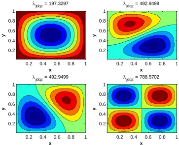
Here A is the Amatrix calculated in a different Matlab script, I is the identity matrix, and 3 is the number of eigenvalues we want to calculate. The more eigenvalues computed, the more one can say about the system. We want to gain information about a small part of the system, hence we choose a small number, i.e. three. We are interested in the smallest eigenvalues for this system, thus we use the ‘sm’ input which gives us the eigenvalues of smallest magnitude.

(21)

21 Figure 5: Results of the eigenfunctions with the four smallest corresponding eigenvalues stated above each graph, whereas the upper left contains the smallest and the lower left contains the highest eigenvalue. Red points have a positive value and the blue points have a negative value.

The figure shows us the results for the eigenfunctions with different eigenvalues. The smallest eigenvalue shows us one peak, how more red the point is, the higher the positive value for that specific point of the eigenfunction is. Also, vise versa, the bluer a point is, the lower its negative value is. The higher the eigenvalue becomes the more peaks the eigenfunctions gets, this due to the eigenfunction being of a wave form. The higher the eigenvalue, the wider the range and thus more periods fit into this range and therefore we get more peaks. Finally when we use the maximum value for the eigenvalue we get a graph such as in figure 2.

4.3 Convergence

The input of our script is of importance for the results we get. The higher our and value, the more nodes we get, i.e. the smaller and will get. By this we can derive a smoother function, thus we get a better result for the smallest eigenvalue, i.e. . Due to limits by the use of memory in Matlab, one cannot do such huge test to calculate the value of convergence. This value is the smallest value for the eigenvalues, i.e. the best value. Therefore one can use another formula. By [3, pp 79-81] we can state the next equations to derive the best value, with Q(N) being the factor of convergence, P(N) being the best value for the given values, and Ԑ(N) being the maximum error, respectively.

x

y

_eigs = 197.3297

0.2 0.4 0.6 0.8 1

0.2 0.4 0.6 0.8 1 x y

_eigs = 492.9499

0.2 0.4 0.6 0.8 1

0.2 0.4 0.6 0.8 1 x y

_eigs = 492.9499

0.2 0.4 0.6 0.8 1

0.2 0.4 0.6 0.8 1 x y

_eigs = 788.5702

0.2 0.4 0.6 0.8 1

(22)

22

The results for these functions can be found in the table below. With the first found results, one can calculate a better answer by using the above equations once more. One can clearly see that the factor of convergence is going to and the eigenvalues converges to the value 197.3921.

N (N) Q1(N) P1(N) Q2(N) P2(N) Ԑ(N)

25 197,1520444 50 197,3296782

100 197,3761736 3,8205 197,3916720 200 197,3880696 3,9085 197,3920350

400 197,3910784 3,9538 197,3920813 7,8309 197,3920844 3,0898E-06 Table 2: An overview of the results of the derivation of the value of convergence

4.4 Jacobi-Davidson QR

The Jacobi-Davidson method is another tool to compute eigenvalues for this problem. The style QR of the Jacobi-Davidson solver is based on the standard eigenproblem, the algorithm is based on the iterative construction of the (generalized) partial Schur form [12]. By this another script is used wherein the most important command is the jdqr, which refers to the script of JDQR by [12]. By use of [V,D,flag] = jdqr(A,I,struct('Disp',1,'Precond',A,'Tol', 1e-4),10,'sm'), where A = Amatrix(Nx,Ny), I = speye(M), and M = Nx*Ny, and the same constants used by the eigs function earlier, we get find the ten lowest eigenvalues, from which we sort out the four smallest. The other parameters are used to get more information about the problem which is solved. Using this function and by use of contourf(x,y,Ez)it results in the next graphs in figure 6.

4.5 Permittivity

At ‘Conditions’ we stated that the electrical permittivity is equal to one. This is true for a vacuum. Due to the system using PCs our εr is not equal to one. Our material has rods of dielectric material inside it. Between those rods there is a vacuum permittivity. Due to this our eigenvalues change. The influence on the eigenvalues depends on which nodes are influenced. If the node is at the center of the system it has more influence on the eigenvalues than if the node is at the boundaries. This can clearly been seen at the graphs. The highest values are at the center of the plot, thus at the middle of the system. This means there is a higher value at this point, due to multiplication a difference has more impact at the middle than at a node with a lower value.

(23)

[image:23.595.109.473.80.375.2]

23 Figure 6: Results of the eigenfunctions of the four smallest corresponding eigenvalues which are

stated above each graph.

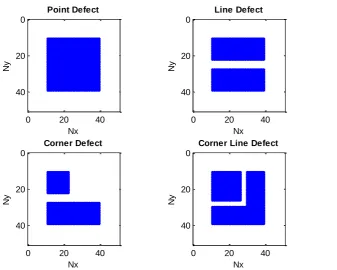
The usefulness of creating a structure with different permittivity leads to different frequency range for the band gap. If adjusted in the right way, one can even, by use of the band gap, steer light. If we use the band gap in such a way that a certain mode can only cross a path and else will be reflected we can send light through a cylinder as described before, but we can also let light make angles of high degrees. By knowing this we have to reset our εr. By [1, p 30] we create a square lattice with the additional rods. The next structures are created shown in figure 7 are created. At these structures the blue dots are equivalent to the rods, with εr equal to 8.9. The white area is the vacuum, with εr equal to 1. The functions are plotted by use of spy(e_rPD), spy(e_rLD)

,

spy(e_rCD), and spy(e_rCLD). A different script is used to plot these graphs, this is left out of this paper due to lack of importance.

Due to the differences in permittivity, the results are influenced, i.e. we get different eigenvalues and thus different graphs.

The eigenfunctions with corresponding eigenvalues, stated above each graph, were plotted in the next graphs. The structures of the grids were one by one implemented in the script. Again by using [V,D,flag] = eigs(A,I,10,'sm') _{the ten smallest eigenvalues for the system were}

calculated, the four smallest eigenvalues were sorted out, which are finally plotted by using contourf(x,y,Ez). This results in the next graphs shown in figures 8, 9, 10, and 11.

x

y

_jdqz = 197.3297

0.2 0.4 0.6 0.8 1

0.2 0.4 0.6 0.8 1 x y

_jdqz = 492.9499

0.2 0.4 0.6 0.8 1

0.2 0.4 0.6 0.8 1 x y

_jdqz = 492.9499

0.2 0.4 0.6 0.8 1

0.2 0.4 0.6 0.8 1 x y

_jdqz = 788.5702

0.2 0.4 0.6 0.8 1

(24)

[image:24.595.147.485.75.345.2]

24 Figure 7: An overview of the set grids with differences in permittivities

Figure 8: Results of the eigenfunctions of the smallest corresponding eigenvalue which is stated above each graph. Each graph has a different grid.

0 20 40

0 20 40 Nx Ny Point Defect

0 20 40

0 20 40 Nx Ny Line Defect

0 20 40

0 20 40 Nx Ny Corner Defect

0 20 40

0

20

40

Nx

Ny

Corner Line Defect

x

y

_PD = 0.81978

0.2 0.4 0.6 0.8 1

0.2 0.4 0.6 0.8 1 x y

_LD = 0.98017

0.2 0.4 0.6 0.8 1

0.2 0.4 0.6 0.8 1 x y

_CD = 1.321

0.2 0.4 0.6 0.8 1

0.2 0.4 0.6 0.8 1 x y

_CLD = 0.92246

0.2 0.4 0.6 0.8 1

(25)

[image:25.595.94.468.78.371.2]

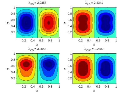
25 Figure 9: Results of the eigenfunctions of the second smallest corresponding eigenvalue which is

stated above each graph. Each graph has a different grid.

Figure 10: Results of the eigenfunctions of the third smallest corresponding eigenvalue which is stated above each graph. Each graph has a different grid.

x

y

_PD = 2.0357

0.2 0.4 0.6 0.8 1

0.2 0.4 0.6 0.8 1 x y

_LD = 2.4341

0.2 0.4 0.6 0.8 1

0.2 0.4 0.6 0.8 1 x y

_CD = 3.3542

0.2 0.4 0.6 0.8 1

0.2 0.4 0.6 0.8 1 x y

_CLD = 2.2887

0.2 0.4 0.6 0.8 1

0.2 0.4 0.6 0.8 1 x y

_PD = 4.0366

0.2 0.4 0.6 0.8 1

0.2 0.4 0.6 0.8 1 x y

_LD = 4.8221

0.2 0.4 0.6 0.8 1

0.2 0.4 0.6 0.8 1 x y

_CD = 6.7709

0.2 0.4 0.6 0.8 1

0.2 0.4 0.6 0.8 1 x y

_CLD = 4.53

0.2 0.4 0.6 0.8 1

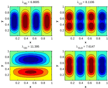
[image:25.595.89.473.430.725.2]

(26)

[image:26.595.112.469.80.371.2]

26 Figure 11: Results of the eigenfunctions of the fourth smallest corresponding eigenvalue which is

stated above each graph. Each graph has a different grid.

By this one can clearly see that a point defect has less influence than for example a corner defect. The differences between the graphs get clearer when we the eigenvalue becomes bigger, i.e. the influences of the grids becomes bigger. Due to the differences in grids the peaks are different shaped and therefore the frequency range of the band gap will become different, and thus different modes, i.e. modes with different frequencies, cannot pass these gaps.

x

y

_PD = 6.8005

0.2 0.4 0.6 0.8 1

x

y

_LD = 8.1106

0.2 0.4 0.6 0.8 1

x

y

_CD = 11.395

0.2 0.4 0.6 0.8 1

x

y

_CLD = 7.6147

0.2 0.4 0.6 0.8 1

(27)

27

5. Results

By use of [20] we implement several matrices which are derived from PCs by use of finite element methods. Due to differences in matrices than used before, the scripts differ from the test cases. The given matrices are way bigger in size compared than used before; therefore the outcomes can be different. Multiple test runs are done to get a better comparison; the multiplicity can differ per test, per preconditioner, and even per solver. The differences in multiplicity are due to the clearance of no improvement or because of saving time. If extra information is stated, this also yields for the larger matrices under the same circumstances.

5.1 First set of matrices

The first set of matrices contains in comparison smaller matrices. The names and sizes are given in the table 3, seen below. Each matrix has a name with n#p#, here n indicates the size and number of elements of the matrix and p indicates the order of the polynomial used for the system, which influences the block size. The N indicates the length of the matrix. The matrix is N x N and has N2 elements.

Matrix N

n1p2 150

n1p3 300

n1p4 525

n2p1 480

n2p2 1200 n2p3 2400 n4p1 3840 n4p2 9600 n8p1 30720 Table 3: Names and Sizes

of the matrices

For this first set of matrices we compare the Eigs function of Matlab and the JDQR function. To compare the functions we call the functions >> [V,D,flag] =

jdqr('matvec_BinvA',N,K,sigma,param_jdqr); and >> Eigenvalues =

(28)

28

n1p2

(N=150)

n1p3

(N=300)

n1p4

(N=525)

Solver JDQR Eigs Solver JDQR Eigs Solver JDQR Eigs

CPU 0,64 0,26 CPU 21,06 0,47 CPU 61,88 0,77

Time 0,56 0,07 Time 22,79 0,44 Time 63,24 0,79

0,63 0,05 25,10 0,41 60,19 0,79

0,58 0,06 22,30 0,46 61,81 0,63

0,49 0,05 19,20 0,37 59,48 0,68

0,59 0,06 25,09 0,41 56,16 0,44

0,55 0,05 19,96 0,51 45,49 0,68

0,52 0,06 22,06 0,31 40,34 1,00

0,63 0,04 19,88 0,39 41,64 0,66

0,55 0,07 18,45 0,49 49,74 0,73

Average 0,57 0,08 Average 21,59 0,43 Average 54,00 0,72

over 5 0,53 0,05 over 5 19,71 0,38 over 5 46,67 0,62

Table 4: Results of first set of matrices; Comparison of Eigs and JDQR

n2p1

(N=480)

n2p2

(N=1200)

n2p3

(N=2400)

CPU 5,49 0,51 CPU 43,04 0,92 CPU 69,73 0,95

Time 4,59 0,45 Time 40,49 0,91 Time 67,20 2,12

4,93 0,45 37,65 0,50 65,96 1,39

4,51 0,15 36,37 0,65 65,47 2,05

4,87 0,42 45,15 0,81 68,29 1,22

5,89 0,47 40,07 0,83 66,42 1,23

5,33 0,22 39,67 0,58 64,52 1,77

6,83 0,41 40,62 0,63 62,48 1,07

6,28 0,52 42,77 0,40 59,75 1,52

6,11 0,25 38,89 0,63 68,81 2,10

over 5 4,85 0,29 over 5 38,53 0,55 over 5 63,64 1,17

(29)

29

n4p1

(N=3840)

n4p2

(N=9600)

n8p1

(N=30720)

CPU 55,28 0,78 CPU 99,19 5,83 CPU 138,13 17,61

Time 36,08 0,82 Time 99,14 6,68 Time 138,97 17,88

58,57 0,88 95,32 5,93 142,96 19,54

55,57 0,83 98,77 6,11 145,59 20,66

59,82 0,78 104,15 5,42 138,84 19,38

48,23 0,79 104,36 5,25 151,79 19,12

51,15 1,85 100,01 5,84 137,83 19,48

65,18 1,92 101,94 6,35 150,14 19,57

56,19 1,46 108,40 5,16 143,12 17,17

45,24 1,38 103,43 6,37 140,70 16,98

over 5 47,20 0,80 over 5 98,49 5,50 over 5 138,89 17,75

Table 6: Results of first set of matrices; Comparison of Eigs and JDQR

A big difference is easy to notice between the two solvers for the small set of matrices. By knowing this our focus is set on the Eigs solver. Different parameters can be filled out for the usage of Eigs. The one we are interested in is the difference between the Arnoldi way of solving or the Lanczos way. By use of Lanczos a matrix has to be symmetric or Hermitian, which is the case for our problem. To set the difference in the parameters for Eigs we simply use the command Opts.Issym which is set to 0 if we want to use the Arnoldi basis, and it is set to 1 if we want to use the Lanczos basis. Due to the default settings of Eigs, we used Opts.Issym = 0;, hence the above calculations are done by use of the Arnoldi basis. Throughout the tables 7, 8, and 9 one can find the results for these runs.

n1p2

(N=150)

n1p3

(N=300)

n1p4

(N=525)

Opts Arnoldi Lanczos Opts Arnoldi Lanczos Opts Arnoldi Lanczos

CPU 0,26 0,10 CPU 0,47 0,34 CPU 0,77 0,66

Time 0,07 0,04 Time 0,44 0,43 Time 0,79 0,62

0,05 0,05 0,41 0,52 0,79 0,73

0,06 0,04 0,46 0,36 0,63 0,67

0,05 0,05 0,37 0,40 0,68 0,53

0,06 0,04 0,41 0,50 0,44 1,08

0,05 0,04 0,51 0,31 0,68 0,73

0,06 0,05 0,31 0,55 1,00 0,55

0,04 0,04 0,39 0,60 0,66 0,71

0,07 0,06 0,49 0,70 0,73 0,82

over 5 0,05 0,04 over 5 0,38 0,37 over 5 0,62 0,61

(30)

30

n2p1

(N=480)

n2p2

(N=1200)

n2p3

(N=2400)

Opts Arnoldi Lanczos Opts Arnoldi Lanczso Opts Arnoldi Lanczos

CPU 0,51 0,43 CPU 0,92 0,67 CPU 0,95 1,78

Time 0,45 0,35 Time 0,91 0,71 Time 2,12 1,89

0,45 0,40 0,50 0,68 1,39 1,85

0,15 0,55 0,65 0,75 2,05 1,75

0,42 0,38 0,81 0,44 1,22 1,67

0,47 0,67 0,83 0,88 1,23 1,65

0,22 0,51 0,58 0,75 1,77 1,63

0,41 0,60 0,63 0,46 1,07 1,64

0,52 0,57 0,40 0,64 1,52 1,62

0,25 0,46 0,63 0,75 2,10 1,65

over 5 0,29 0,40 over 5 0,55 0,58 over 5 1,17 1,64

Table 8: Results of first set of matrices; Comparison of Arnoldi and Lanczos

n4p1

(N=3840)

n4p2

(N=9600)

n8p1

(N=30720)

Opts Arnoldi Lanczos Opts Arnoldi Lanczos Opts Arnoldi Lanczos

CPU 1,71 0,80 CPU 5,83 6,15 CPU 17,61 16,96

Time 1,36 1,86 Time 6,68 5,46 Time 17,88 17,47

0,83 1,77 5,93 5,63 19,54 19,47

1,90 1,58 6,11 5,19 20,66 17,82

1,96 1,07 5,42 6,07 19,38 16,67

1,85 1,18 5,25 6,44 19,12 16,57

1,67 1,75 5,84 4,95 19,48 16,23

1,71 1,46 6,35 4,88 19,57 16,59

1,49 0,80 5,16 5,63 17,17 16,37

1,13 2,03 6,37 6,13 16,98 16,31

over 5 1,30 1,06 over 5 5,50 5,22 over 5 17,75 16,41

Table 9: Results of first set of matrices; Comparison of Arnoldi and Lanczos

5.2 Second set of matrices

(31)

31 of the same names and sizes as for the first set of matrices, these matrices are computed in a

different way and therefore are tested over again.

Matrix N

n2p1 480

n2p2 1200 n2p3 2400 n4p1 3840 n4p2 9600 n4p3 19200 n8p1 30720 n8p2 76800 n8p3 153600 n16p1 245760 n16p2 614400 n32p1 1966080 Table 10: Names and

sizes of the matrices

Also, for this second set of matrices we compare the Eigs function of Matlab and the JDQR function. The same situation is taken as before. We call the functions >> [V,D,flag] =

jdqr('matvec_BinvA',N,K,sigma,param_jdqr); and >> Eigenvalues =

(32)

32

n2p1

(N=480)

n2p2

(N=1200)

n2p3

(N=2400)

CPU 4,77 0,65 CPU 31,83 1,70 CPU 65,21 2,54

Time 5,66 0,32 Time 33,42 0,90 Time 59,47 3,26

5,67 0,64 30,40 1,55 60,86 2,66

4,36 0,50 32,28 0,80 60,68 3,12

3,63 0,63 28,39 1,45 63,39 2,30

4,86 0,67 28,95 0,68 67,71 2,86

3,94 0,64 33,08 1,34 61,80 2,06

5,53 0,85 33,18 1,99 64,27 2,70

4,70 0,73 33,19 1,18 63,81 3,12

5,05 0,67 32,80 1,82 63,73 2,32

over 5 4,28 0,55 over 5 30,37 0,98 over 5 61,24 2,38

Table 11: Results of second set of matrices; Comparison of Eigs and JDQR

n4p1

(N=3840)

n4p2

(N=9600)

n4p3

(N=19200)

CPU 21,90 4,69 CPU 62,49 34,29 CPU 242,38 76,03

Time 20,22 4,16 Time 58,07 32,87 Time 229,72 70,11

21,73 4,92 58,91 165,58 232,46 75,71

15,00 3,84 57,32 37,72 229,44 73,33

25,05 4,02 61,43 32,26 240,50 99,85

27,79 3,94 60,72 44,79 217,31 78,36

21,73 3,83 58,55 31,58 228,77 75,57

21,13 3,66 54,56 38,55 227,58 74,43

28,26 4,34 55,64 184,37 237,90 104,03

18,99 3,84 57,29 30,82 242,14 133,60

over 5 19,41 3,82 over 5 56,58 32,36 over 5 226,56 73,83

(33)

33

n8p1

(N=30720)

n8p2

(N=76800)

n8p3

(N=153600)

CPU 88,05 110,71 CPU 526,49 2040,20 CPU 1662,60 2667,70

Time 94,02 122,51 Time 475,24 1333,20 Time 1683,50 2696,10

95,90 120,90 529,60 1294,80 1645,00 3328,90

61,27 114,41 533,89 1637,60 1688,20 2798,70

81,94 121,70 519,73 1616,20 1645,90 3320,80

93,59 121,32 516,00 2125,50 1648,50 2709,20

87,29 105,06 517,54 1969,00 1643,70 3842,40

86,04 111,78 511,75 1904,40 1672,40 2792,80

95,84 108,97 515,87 1817,00

62,28 113,09 533,92 1501,70

Average 84,62 115,05 Average 518,00 1723,96 Average 1661,23 3019,58 over 5 75,76 109,92 over 5 507,28 1476,70 over 5 1649,14 2732,90

n16p1

(N=245760)

n16p2

(N=614400)

n32p1

(N=1966080)

CPU 755,25 8427,10 CPU 3847,50 CPU 18312,00

Time 890,17 5177,80 Time 3792,20 error Time 18535,00 error

789,45 5846,50 2805,40 sparse lu 20629,00 sparse lu

831,00 5982,10 3767,60 UMFPACK UMFPACK

703,66 6312,00 3863,40 failed no eigen- failed

721,55 5195,20 3837,00 values

846,30 4992,70 3765,90 found

681,57 5442,30 3839,50 within

300

iterations

Average 777,37 5921,96 Average 2951,85 Average 19158,67

over 5 730,30 5330,90 over 5 3593,62 over 5 0,00

A change can be clearly seen between the smaller and larger matrices. The JDQR solver becomes faster than the Eigs solver for matrices bigger than or equal to n8p1, i.e. for . Thus our focus is set on the JDQR solver. There are several more ways to improve the running time. The above runs were all solved by use of the ‘normal’ way of solving the inverse of the matrix, which is with the backslash (\) operator of Matlab. We used the next script, which is stated as BinvA:

>> function y = matvec_BinvA(x) >> global A B

(34)

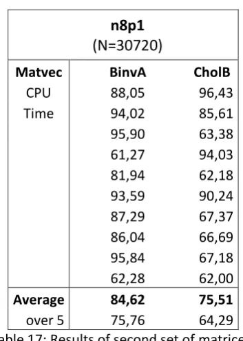
34 Another way to solve the problem is to change the way of solving the inverse of A. By this we do not use the back slash operator of Matlab for the given matrices. We first take the Cholesky factorization of B and than solve the equation. By this we need to take the inverse, i.e. back slash operator, of the factorized matrices, which can lead to an improvement of running time. We used the following script, which is stated as CholB:

>> function y = matvec_BinvA(x) >> global A B

>> [R p S] = chol(B);

>> y = S*(R\(R'\(S'*(A*x))));

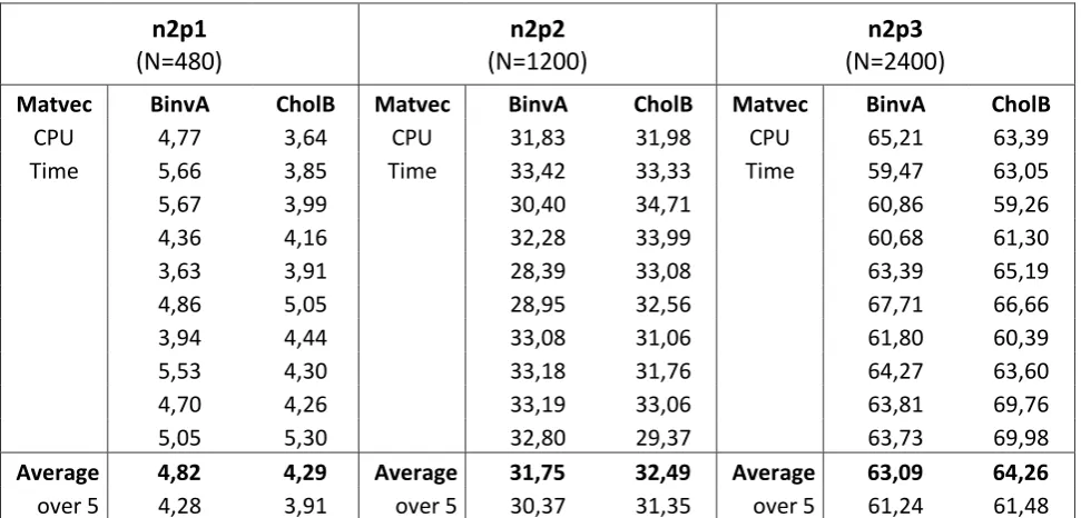
Throughout the tables 15, 16, and 17 the results can be found. These tests are not done for all the matrices due to comparison of the matrices itself. The only difference can be found in the

computation of matrix, thus not all matrices have to be tested to get to the conclusion.

n2p1

(N=480)

n2p2

(N=1200)

n2p3

(N=2400)

Matvec BinvA CholB Matvec BinvA CholB Matvec BinvA CholB

CPU 4,77 3,64 CPU 31,83 31,98 CPU 65,21 63,39

Time 5,66 3,85 Time 33,42 33,33 Time 59,47 63,05

5,67 3,99 30,40 34,71 60,86 59,26

4,36 4,16 32,28 33,99 60,68 61,30

3,63 3,91 28,39 33,08 63,39 65,19

4,86 5,05 28,95 32,56 67,71 66,66

3,94 4,44 33,08 31,06 61,80 60,39

5,53 4,30 33,18 31,76 64,27 63,60

4,70 4,26 33,19 33,06 63,81 69,76

5,05 5,30 32,80 29,37 63,73 69,98

[image:34.595.56.542.314.547.2]

over 5 4,28 3,91 over 5 30,37 31,35 over 5 61,24 61,48

(35)

35

n4p1

(N=3840)

n4p2

(N=9600)

n4p3

(N=19200)

Matvec BinvA CholB Matvec BinvA CholB Matvec BinvA CholB

CPU 21,90 20,36 CPU 62,49 61,26 CPU 242,38 234,55

Time 20,22 14,57 Time 58,07 59,02 Time 229,72 239,13

21,73 21,99 58,91 64,47 232,46 241,46

15,00 16,96 57,32 62,42 229,44 240,51

25,05 17,01 61,43 61,61 240,50 237,90

27,79 19,95 60,72 57,41 217,31 236,03

21,73 20,16 58,55 95,16 228,77 247,65

21,13 22,28 54,56 57,44 227,58 239,29

28,26 15,50 55,64 78,98 237,90 240,15

18,99 21,38 57,29 60,19 242,14 240,34

Average 22,18 19,02 Average 58,50 65,80 Average 232,82 239,70

[image:35.595.57.543.65.303.2]

over 5 19,41 16,80 over 5 56,58 59,06 over 5 226,56 237,38

Table 16: Results of second set of matrices; Comparison of BinvA and CholB

n8p1

(N=30720)

Matvec BinvA CholB

CPU 88,05 96,43

Time 94,02 85,61

95,90 63,38

61,27 94,03

81,94 62,18

93,59 90,24

87,29 67,37

86,04 66,69

95,84 67,18

62,28 62,00

Average 84,62 75,51

over 5 75,76 64,29

Table 17: Results of second set of matrices; Comparison of BinvA and CholB

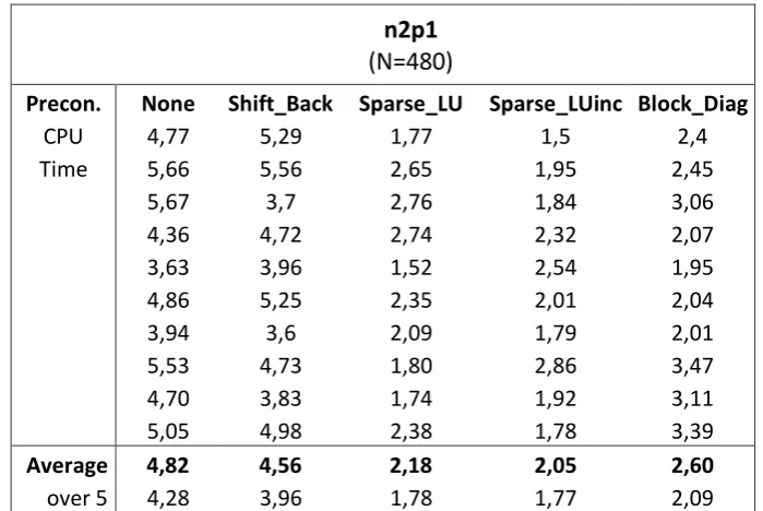
[image:35.595.208.385.348.596.2]

(36)

36

n2p1

(N=480)

Precon. None Shift_Back Sparse_LU Sparse_LUinc Block_Diag

CPU 4,77 5,29 1,77 1,5 2,4

Time 5,66 5,56 2,65 1,95 2,45

5,67 3,7 2,76 1,84 3,06

4,36 4,72 2,74 2,32 2,07

3,63 3,96 1,52 2,54 1,95

4,86 5,25 2,35 2,01 2,04

3,94 3,6 2,09 1,79 2,01

5,53 4,73 1,80 2,86 3,47

4,70 3,83 1,74 1,92 3,11

5,05 4,98 2,38 1,78 3,39

Average 4,82 4,56 2,18 2,05 2,60

[image:36.595.122.472.69.303.2]

over 5 4,28 3,96 1,78 1,77 2,09

Table 18: Results of second set of matrices; Comparison of preconditioners for JDQR

n2p2

(N=1200)

CPU 31,83 21,29 7,39 7,2 11,58

Time 33,42 21,42 9,43 6,25 7,49

30,40 20,24 9,51 6,93 8,70

32,28 17,92 7,68 6,61 10,22

28,39 17,72 7,72 8,66 8,99

28,95 20,37 7,65 7,43 10,59

33,08 19,15 9,03 6,81 10,39

33,18 19,09 8,56 7,2 11,57

33,19 17,17 7,78 7,24 11,29

32,80 19,33 6,07 5,44 9,20

Average 31,75 19,37 8,08 6,98 10,00

over 5 30,37 18,21 7,30 6,41 8,92

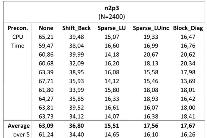
[image:36.595.123.474.355.587.2]

(37)

37

n2p3

(N=2400)

CPU 65,21 39,48 15,07 19,33 16,47

Time 59,47 38,04 16,60 16,99 16,76

60,86 39,99 14,18 20,67 20,62

60,68 32,09 16,20 18,13 20,34

63,39 38,95 16,08 15,58 17,98

67,71 35,93 14,12 15,46 13,69

61,80 33,99 15,80 18,08 18,01

64,27 35,85 16,33 18,93 16,42

63,81 39,52 16,61 16,07 18,00

63,73 34,12 14,07 16,38 18,41

Average 63,09 36,80 15,51 17,56 17,67

[image:37.595.121.472.69.303.2]

over 5 61,24 34,40 14,65 16,10 16,26

n4p1

(N=3840)

CPU 21,90 26,88 9,45 14,53 11,65

Time 20,22 23,77 7,45 11,67 11,2

21,73 26,89 10,65 12,98 11,23

15,00 23,83 9,69 13,09 12,39

25,05 23,87 8,76 12,98 12,5

27,79 22,22 10,09 12,82 11,49

21,73 28,12 8,46 13,3 11,01

21,13 25,85 9,46 11,05 11,19

28,26 18,03 10,04 12,67 13,06

18,99 22,88 7,14 12,66 12,83

Average 22,18 24,23 9,12 12,78 11,86

over 5 19,41 22,15 8,25 12,17 11,22

[image:37.595.121.471.354.588.2]

(38)

38

n4p2

(N=9600)

CPU 62,49 129,42 42,14 92,32 58,76

Time 58,07 137,09 41,39 100,56 55,20

58,91 139,47 40,97 93,73 52,76

57,32 145,35 42,30 97,97 60,48

61,43 124,48 38,14 94,07 58,73

60,72 146,47 43,90 54,83

58,55 110,39 42,31 55,39

54,56 126,58 40,82 55,89

55,64 125,17 40,76 61,31

57,29 137,66 41,18 57,53

Average 58,50 132,21 41,39 95,73 57,09

[image:38.595.121.472.69.303.2]

over 5 56,58 123,21 40,37 95,73 54,81

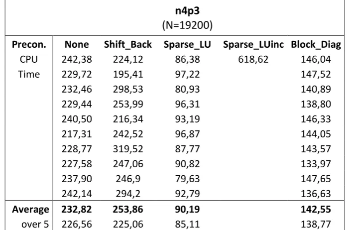
n4p3

(N=19200)

CPU 242,38 224,12 86,38 618,62 146,04

Time 229,72 195,41 97,22 147,52

232,46 298,53 80,93 140,89

229,44 253,99 96,31 138,80

240,50 216,34 93,19 146,33

217,31 242,52 96,87 144,05

228,77 319,52 87,77 143,57

227,58 247,06 90,82 133,97

237,90 246,9 79,63 147,65

242,14 294,2 92,79 136,63

Average 232,82 253,86 90,19 142,55

over 5 226,56 225,06 85,11 138,77

[image:38.595.122.471.353.584.2]

(39)

39

n8p1

(N=30720)

CPU 88,05 338,38 113,30 555,54 261,19

Time 94,02 285,26 113,10 265,11

95,90 339,49 110,40 264,76

61,27 317,39 114,73 269,59

81,94 382,18 126,61 259,95

93,59 292,42 112,63 263,72

87,29 392,49 124,81 260,24

86,04 347,1 108,24 264,3

95,84 347,42 118,44 267,03

62,28 288 115,24 267,49

Average 84,62 333,01 115,75 264,34

[image:39.595.121.472.69.303.2]

over 5 75,76 304,29 111,53 261,88

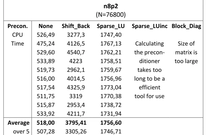
n8p2

(N=76800)

Precon. None Shift_Back Sparse_LU Sparse_LUinc Block_Diag CPU 526,49 3277,3 1747,40

Time 475,24 4126,5 1767,13 Calculating Size of 529,60 4540,7 1762,21 the precon- matrix is

533,89 4223 1758,51 ditioner too large

519,73 2962,1 1759,67 takes too

516,00 4014,5 1756,96 long to be a

517,54 4325,9 1773,04 efficient

511,75 3319 1770,38 tool for use

515,87 2953,4 1738,72

533,92 4211,7 1731,94

Average 518,00 3795,41 1756,60

over 5 507,28 3305,26 1746,71

[image:39.595.121.475.356.587.2]

(40)

40

n8p3

(N=153600)

Solver None Shift_Back Sparse_LU Sparse_LUinc Block_Diag CPU 1662,60 6565,90 2576,59

Time 1683,50 2703,52

1645,00 2567,03

1688,20 2545,10

1645,90 2737,57

1648,50 2450,58

1643,70 2516,21

1672,40 2554,46

2644,75

2477,57

Average 1661,23 2577,34

[image:40.595.123.474.69.302.2]

over 5 1649,14 2508,78

n16p1

(N=245760)

Solver None Shift_Back Sparse_LU Sparse_LUinc Block_Diag CPU 755,25 1255,1 4436,56

Time 890,17 4370,79

789,45 4216,32

831,00 4370,94

703,66 4386,41

721,55 4311,41

846,30 4241,66

681,57 4423,77

4399,99

4261,12

Average 777,37 4341,90

over 5 730,30 4280,26

[image:40.595.120.476.353.584.2]

(41)

41

n16p2

(N=614400)

Precon. None Shift_Back Sparse_LU Sparse_LUinc Block_Diag CPU 3847,50

Time 3792,20 out of error

2805,40 memory UMFPACK

3767,60 failed

3863,40

3837,00

3765,90

3839,50

Average 3689,81

[image:41.595.118.479.69.302.2]

over 5 3593,62

n32p1

(N=1966080)

Precon. None Shift_Back Sparse_LU Sparse_LUinc Block_Diag CPU 18312,00

Time 18535,00

20629,00

no eigen-

values

found

within

300

iterations

Average 19158,67

over 5

[image:41.595.114.481.352.586.2]

(42)

42

Iterations

Size None Shift_Back Sparse_LU Sparse_LUinc Block_Diag

n2p1 96 74 42 41 40

n2p2 242 80 53 49 52

n2p3 300 78 58 53 53

n4p1 88 62 36 39 37

n4p2 184 65 38 42 52

n4p3 300 56 44 40 55

n8p1 135 60 44 48 47

n8p2 297 62 42

n8p3 300 89 40

n16p1 266 45

n16p2 300

[image:42.595.125.474.69.287.2]

n32p1

Table 30: Results of second set of matrices; Comparison of number of iterations needed

Here one can clearly see that the preconditioner does improve the number of iterations needed, but per iterations step it takes more time to solve.

For comparison of the preconditioners in table 31 an overview is made in how long it takes for the preconditioner to be calculated. By this we can compare how long it takes for the overall problem to be solved after the preconditioner is calculated.

CPU Precon.

Size None Shift_Back Sparse_LU Sparse_LUinc Block_Diag

n2p1 0 0,01 0,04 0,03 0,06

n2p2 0 0,03 0,08 0,52 0,12

n2p3 0 0,10 0,36 5,12 0,35

n4p1 0 0,08 0,22 5,15 0,30

n4p2 0 0,86 2,95 82,94 3,47

n4p3 0 1,89 6,55 596,97 7,73

n8p1 0 3,16 12,08 526,03 14,23

n8p2 0 55,95 205,89

n8p3 0 117,79 434,27

n16p1 0 894,12

n16p2 0

n32p1 0

[image:42.595.113.486.462.677.2]

Comparison of iterative eigenvalue solvers for photonic crystal modeling