Numerical Simulation over a backward facing step with OpenFOAM

(1)

University of Twente

Internship at CIRA

Numerical Simulation over a backward facing step

with OpenFOAM

Author

:

Arjan Slaper

August 24, 2014

CIRA supervisor

:

Dr. E. Iuliano

(2)

Preface

From February to May 2014, I have done my internship at CIRA in Italy for my Mechanical Engineering master in Engineering Fluid Dynamics. Over these couple of months I have experienced an entirely different working and living environment. I enjoyed it very much and learned a lot.

I would like to thank professor Hoeijmakers for providing me this opportunity and the support for this internship from the Netherlands. From CIRA, I would specially like to thank dr. Emiliano Iuliano for all the help and guidance at CIRA and with the assignment but also for all the help and support outside of the working environment. Fur-thermore I would like to thank my colleagues from CIRA and friends for making this internship a wonderful experience.

(3)

List of Figures

1.1 Turbulence in a wind turbine park [20] . . . 1

1.2 Turbulence found on the weather chart [21] . . . 1

1.3 Energy of a turbulent flow [4] . . . 2

2.1 Reynolds Decomposition [4] . . . 6

2.2 Different filter types in the real space (a) and the Fourier space (b). sharp Fourier cutoff, -truncated Gaussian, -·- top-hat [6] . . . 9

2.3 When to use wall models [14] . . . 10

2.4 Skewness of a cell [19] . . . 13

2.5 A non orthogonal cell [18] . . . 13

2.6 Multi-grid solver with 5 levels . . . 16

3.1 Mesh used in the circular cylinder case ofRe 40 . . . 18

3.2 Convergence for the circular cylinder case withRe 40 . . . 19

3.3 Results for pressure and velocity in the circular cylinder case withRe 40 . . . 19

3.4 Results for pressure distribution at the circular cylinder wall withRe40 . . . 20

3.5 Mesh used for the circular cylinder case with Re106 _{. . . .} ₂₀

3.6 Convergence for the uRANS circular cylinder case withRe 1e6 . . . 21

3.7 Results for pressure and velocity of the circular cylinder case withRe 1e6 . . . 22

3.8 Results for pressure distribution at the circular cylinder wall withRe1e6 with the ones of the paper [13] 22 3.9 Results for velocity distribution in the circular cylinder case withRe 1e6 and the results of the paper [13] 23 3.10 Results for lift and drag coefficient of the circular cylinder case atRe 1e6 . . . 23

3.11 Mesh used for the LES circular cylinder case with Re106 . . . 24

3.12 Convergence for the LES circular cylinder case withRe1e6 . . . 25

3.13 Average bubble shape of the circular cylinder LES case forRe 1e6. . . 25

3.14 Results for pressure distribution at the circular cylinder wall withRe 1e6in LES case with the ones of the paper [13] . . . 25

3.15 Velocity distribution in the LES circular cylinder case withRe 1e6 and the results of the paper [13] . . 26

3.16 Results for lift and drag coefficient of the circular cylinder case atRe 1e6 . . . 26

3.18 Distribution of the blocks over the backward facing step. . . 28

3.19 The used grid . . . 29

3.20 Velocity profile atx/h=−0.35for the steady case . . . 30

3.21 ˜ν profile atx/h=−0.35 for the steady case . . . 30

3.22 Zoom of the coarse mesh. . . 31

3.23 Residuals of the coarse mesh backward facing step simulation . . . 32

3.24 Velocity profile at station x_h =−0.43 . . . 32

3.25 . . . 33

3.26 . . . 34

3.27 . . . 34

3.28 . . . 35

3.29 Area where the mean velocity inx-direction is negative forming the bubble . . . 35

(5)

List of Tables

3.1 Summary results ofRe 40 [8] . . . 20

3.2 Boundary conditions for the circular cylinder case atRed= 1e6 . . . 21

3.3 Summary results ofRe 1e6, computations from the paper and experiments [13] . . . 22

3.4 Boundary conditions for the LES circular cylinder case atRed= 1e6 . . . 24

3.5 Inflow and outflow conditions for the backward facing step. . . 27

3.6 Cell distribution in the backward facing step . . . 29

3.7 Boundary conditions for the IDDES simulation . . . 29

(6)

1

Introduction

1.1 CIRA

The Centro Italiano Ricerche Aerospaziali or CIRA is the largest aerospace research facility in Italy. It was founded in 1984 and is a corporation with private and public shareholders who are all interested in the same goal: improvement in aeronautical and space engineering. Together with the European Space Agency, they managed to the build many unique testing facilities as for example an icing wind tunnel and a plasma wind tunnel. There are currently about 350 people working for CIRA.

The icing wind tunnel of CIRA is the biggest icing wind tunnel in the world. There are different test sections which can be used to test either scale models or even complete parts of an airplane at altitudes up to 7000 meters, speeds of 800 km/h and temperatures up to−40 degrees Celsius.

The plasma wind tunnel is used to test the heat protection systems of re-entry vehicles. Objects with a diameter up to 2 meter can be put into the test section where temperatures up to 10.000 degrees Celsius can be reached. Because of the size of the objects and conditions the objects can be tested in, this facility is unique in the world.

At CIRA, there are also testing facilities for testing safety systems during air crashes as well as transonic and hypersonic wind tunnels. With all these facilities, it is possible for CIRA to do a wide variety of tests for all kinds of aerospace companies.

Besides all these testing facilities, CIRA also has a devision for computational fluid dynamics. All kinds of problems are examined here from icing problems to optimization problems as well as calculations on the re-entry vehicle which is currently under development.

1.2 Turbulence

When people are asked about turbulence, many will think about airplanes and the uncomfortable situations turbulence causes during flight. It will take a lot more thinking for most people to realize that turbulence is everywhere around us. The path of smoke coming from a cigarette or chimney, the flow of water from a fountain and the weather are all examples of situations where turbulence is encountered in our daily lives.

Figure 1.1: Turbulence in a wind turbine park [20] _{Figure 1.2:} _{Turbulence found on the weather chart [21]}

(7)

The main predictor of turbulent behaviour is the Reynolds number. The Reynolds number (as defined in 1.1) is the relation between the viscous forces and the inertial forces. In low Reynolds number flows the flow is laminar and the viscosity plays an important role, while in high Reynolds number flows the influence of the viscous forces is very small in comparison to the inertial forces and the flow becomes turbulent.

Re= ρU L

µ (1.1)

When a turbulent flow is studied, the structures observed are irregular both in space and time (see the structures in figures 1.1 and 1.2 as examples). This irregularity causes a lot of problems in the calculations of turbulent flow problems and the design processes. The turbulent structure at one time instant is very chaotic and this behaviour does not improve if the time is advanced. A turbulent flow is different at every spatial place and time instant. Because of this behaviour, it is very difficult to predict where a certain particle will end up. With experiments it was tried to find the flow path of a particle in a turbulent flow. It turned out that it was impossible to predict the exact location because the trajectory of the particle depends both on its position in space as well as in time. A small change in the initial condition will result in a totally different end position of the particle. The approach of trying to predict the path of each individual particle did not work out for a design process. It turned out, however, that it was possible to extract some statistics from the flow. These statistics, in the form of probability density functions, could be used to extract general behaviour of the flow particles and of the flow in general. When a turbulent flow field at a certain time instant is studied more carefully, it can be seen that it contains all kinds of eddies which contain eddies within itself. Lewis Richardson summarized the process of a turbulent flow in one of his papers written in 1922 as:

Big whorls have little whorls That feed on their velocity, And little whorls have lesser whorls

And so on to viscosity.

Figure 1.3: Energy of a turbulent flow [4]

This poem describes the energy cascade through all the length scales up to a length scale where the viscosity be-comes dominant again and the energy dissipates. The energy of each size of eddies can be plotted as function of the wave length as is done in figure 1.3. It shows that the big eddies contain the most energy and that the amount of energy of the flow decays through the flow regime. It was Kolmogorov who defined the length scale in the tur-bulent process at which the energy is dissipated through the viscosity. He stated that the bigger scales are not dependent of the viscosity and only dependent on the en-ergy dissipation. The smallest eddies dependent on the dissipation and the viscosity. These statements were pre-sented in 1941 so that is why this theory is called the K41 hypothesis. He also stated that the different eddy lengths all behave in a similar fashion and that scale similarity can be used in order to predict certain behaviours for certain eddy sizes. This similarity hypothesis describes that the energy is only dependent of the dissipation ratio and not of the viscosity for the larger sized eddies. The smallest scales are influenced by the dissipation as well as the viscosity.

(8)

τi,j = 2µtSi,j∗ − 2 3ρkδi,j

−u0

iu0j =νt

_∂U

i

∂xj +∂Uj

∂xi

−2

3

∂Uk

∂xk

δi,j

−2

3kδi,j

(1.2)

In the second half of the 20th century the computer power increased rapidly. This resulted in many new possibilities such as the moon landing but also the research in a lot of different fields including turbulence. The research in turbu-lence got a boost because the computer could be used to help the understanding of turbuturbu-lence. Many different models and methods were developed in order to try and predict turbulent behaviour in all kind of different environments and designs. These models were tested using various different test cases and setups.

(9)

2

Fluid flow and modeling

2.1 The Navier-Stokes equations

The Navier-Stokes equations describe the motion of fluids and fluid-like substances. These equations form the basis for every analysis, design or production process of any kind of machine which has something to do with fluid flow. The Navier-Stokes equations (given in integral conservation form in 2.1) are the conservation laws for mass, momentum and energy. In order to apply these equations, it has to be assumed that the fluid is a continuum, uniform and homogeneous of composition.

∂ ∂t ˚ V ρdV + ¨ ∂V

ρ(~u−u~∂V)·~ndS= 0

∂ ∂t

˚

V

ρ~udV + ¨

∂V

ρ~u[(~u−u~∂V)·~n]dS= ˚

V

ρ ~f dV −

¨

∂V

p~ndS+ ¨

∂V

τ·~ndS ∂ ∂t ˚ V ρEdV + ¨ ∂V

ρE(~u−u~∂V)·~ndS= ˚

V

ρ~u·f dV~ −

¨

∂V

p~u·~ndS+ ¨

∂V

τ ~u

·~ndS+ ˚ V ˙ QdV − ¨ ∂V ~ u·~ndS

(2.1)

These equations can also be rewritten into the PDE (partial differential equation) non-conservation form resulting in 2.2.

Dρ

Dt +ρ ~∇ ·~u= 0 ρD~u

Dt =ρ ~f− ~

∇p+∇ ·~ τ ρDE

Dt =ρ~u· ~

f−∇ ·~ (τ ~u) + ˙Q−∇ ·~ ~q

(2.2)

For the problems described in this report, the main focus will be on the mass and momentum equation and the application of these two equations since the problems described here do not involve heat transport. When these two vector equations are put into the Einstein notation, the following can be obtained:

∂ρ ∂t +ui

∂ρ ∂xi

+ρ∂ui ∂xi

= 0

∂ρui

∂t + ∂ρujui

∂xj

=ρfi−

∂p ∂xi

+∂τj,i

∂xj

(2.3)

In the momentum equation, the term ∂τj,i

∂xj represents the viscous stresses in the flow and the tensor τi,j is assumed

to be symmetric. The fluids considered in this report are also considered Newtonian fluids. This assumptions means that the viscous stresses are assumed proportional to the rate of strain resulting in the expression given in 2.4 [1].

τi,j =µ

_∂u

i

∂xj +∂uj

∂xi

Withµbeing the viscosity

(2.4)

(10)

∂ρ ∂t +ui

∂ρ ∂xi

+ρ∂ui ∂xi

= 0

∂ρui

∂t + ∂ρujui

∂xj

=ρfi−

∂p ∂xi + ∂ ∂xj µ _∂u j ∂xi + ∂ui

∂xj

=ρfi−

∂p ∂xi

+µ _∂2_u

j

∂xi∂xj

+ ∂

2_u

i

∂xj∂xj

(2.5)

In case of an incompressible flow (which will be the case for the studied cases in this report), the equations reduce to 2.6.

∂ui

∂xi = 0

And directly applied to the momentum equation:

∂ui

∂t + ∂ujui

∂xj

=fi− 1 ρ ∂p ∂xi +µ ρ ∂2ui

∂xj∂xj

=fi− 1

ρ ∂p ∂xi

+ν ∂

2_u

i

∂xj∂xj

withν being the kinematic viscosity

(2.6)

2.2 Modeling of the Navier Stokes equations

To use computer models as an analysis tool, a model is required to give a good approximation of the reality within a reasonable time frame. It is exactly this principle that causes the large variety in models and methods applied in CFD codes. For some purposes it can be good to have a quick solution and the accuracy is not so important while in other cases accuracy is more important. Because of this, there is a wide range of CFD codes, models and methods to solve for different flow simulations.

2.2.1 OpenFOAM

The program used to solve the different flow problems in this report is OpenFOAM. OpenFOAM is a free open source CFD package and can be downloaded from their website [15]. It is developed by OpenCFD Ltd and distributed by the OpenFOAM foundation. It is widely applicable because of the many different solvers implemented in the software. The software package can be used in both commercial and academic organizations to solve all types of problems (from complex flows with chemical reactions to turbulence and from electromagnetics to financial problems). The wide applicability of this package is caused by the ability of the software to solve partial differential equations very efficiently. The package is constantly developed not only by the people behind the code but also by users from all over the world.

The package includes software from the preprocessing up to the post processing processes. The package contains over 80 solver applications for different types of problems and over 170 utility applications that perform the pre- and post-processing tasks. [15].

One of the major advantages of OpenFOAM is the ability to run processes in parallel which greatly improves the speed of the calculations and processing of large amounts of data. Because there are so many different solvers and techniques implemented, it is very easy to switch in order to improve the quality of the results or to get a stable run for example.

2.2.2 Turbulence modeling techniques

(11)

Direct Numerical Simulation

Direct Numerical Simulation (DNS) solves the Naviers-Stokes equations for every scale that is present in the fluid motion. This results in a very accurate solution of the flow since only some numerical errors are introduced. In order to get a very accurate result, the grid used for DNS has to be fine enough to resolve the turbulent motion from the large motion scales on to the order of the Kolmogorov scale [3]. This means that in case of difficult geometries, the grid is very difficult to construct and extremely big. Because DNS is a very demanding process, it could only be applied from the 1970’s because sufficient amount of computer power was available from that time on. It has been estimated that the computational cost scale with Re3 [2] which makes this method not applicable in high Reynolds number flows because the time it takes to find a solution will be too long.

This method can be used in order to understand turbulence and to extract statistical data which can not easily be found in experiments. For example, it helped to quantify the influence of the tools used in measurements and helped to find better measurements methods [3].

DNS is an extremely interesting tool to analyze and understand turbulence better. In a design process however, this method is too demanding in order to be used effectively.

Reynolds-Averaged Navier-Stokes equations

Figure 2.1: Reynolds Decomposition [4]

Method A different technique to solve the Navier Stokes equation is the Reynolds-Averaged Navier-Stokes method or RANS method. This method is developed in order to find a suitable solution in a flow problem within a very reasonable time. This means that it will not solve the Navier Stokes equations exactly but will apply a model in order to come to a solution. A RANS solver uses Reynolds decomposition and the time-averaged Navier-Stokes equations. The main assumption in Reynolds de-composition is that the variables, which are solved, can be split into two parts, the first being the mean quan-tity and the second being a variation. This principle is shown for the velocity in figure 2.1 and in general in 2.7. It should be noted that ¯.represents the mean value.

~

φ=φ~+φ~0

(2.7)

With the use of the Reynolds decomposition of 2.7 and the Navier-Stokes equations in 2.6, a set of Reynolds decomposed Navier-Stokes equations can be defined as in 2.8.

∂ ∂xi

(ui+u0i) =

∂ ∂xi

ui+

∂ ∂xi

u0_i= 0

∂

∂t(ui+u

0

i) +

∂ ∂xj

(ui+u0i)(uj+u0j) =

∂

∂t(ui+u

0

i) +

∂ ∂xj

(uiuj+u0iuj+uiu0j+u

0

iu

0

j)

= (f_i+f_i0)−1

ρ ∂ ∂xi

(p_i+p0_i) +ν ∂

2

∂xj∂xj

(ui+u0i)

(2.8)

The time average of a variable will result in the mean value of that same variable. It can be shown that the time average of the fluctuations is equal to zero as is done in 2.9. The time average of the mass conservation equation (2.8) is taken. In 2.9,h.iis the time average.

_∂ ∂xi ui + _∂ ∂xi

u0_i

= ∂

∂xi

ui = 0

and from 2.8

∂ ∂xi

u0i= 0

(2.9)

(12)

_∂

∂t(ui+u

0 i) + _∂ ∂xj

(uiuj+u0iuj+uiu0j+u

0 iu 0 j) =

(f_i+f_i0)

−

₁

ρ ∂ ∂xi

(p_i+p0_i)

+

ν ∂

2

∂xj∂xj

(ui+u0i)

∂ ∂t(ui) +

∂ ∂xj

(uiuj) =fi− 1

ρ ∂pi

∂xi +ν ∂

2_u

i

∂xj∂xj

− ∂

∂xj

u0_iu0_j

(2.10)

The equations in 2.9 and 2.10 form the Unsteady Reynold-Averaged Navier-Stokes equations or uRANS equations. There are two basic arguments for keeping the time derivative in these equations. The first one has to do with the ergodicity of the equaions which states that the time averaging is equal to the ensemble averaging. The second has to do with the fact that there are multiple time scales where it is stated that there are two time scales, a large and a small for where the average is taken over the small time scale and the large time scale fluctuations are kept. There are some arguments for and opposed to these hypothesis and more information can be found in [4].

The last term in the second equation in 2.10 represent the so-called Reynold stresses (to make it a true stress, it should be multiplied with ρ, but this was already divided out since it was assumed to be constant). The Reynold Stress represents the transport of momentum through the turbulent nature of the flow.

The equation of momentum as given in 2.10 represents three independent equations. Together with either the conser-vation of mass (equation in 2.9) or the Poisson equation, the total of independent equations adds up to 4. However when the number of unknowns is counted, it can be seen that with the three components of velocity, pressure and the Reynold Stresses, it exceeds the number of independent equations (assuming the other forces are given). This problem is called the closure problem [2]. It is because of this closure problem that the uRANS-equations require some sort of model for the Reynold Stress. Many different models were developed in order to solve this part of the equations, however it is very difficult to find a suitable model. A few of these models will be explained later on.

Models There are many different models used to describe the Reynolds stress. The most simple model would be an algebraic solver which calculates the magnitude of the Reynolds stress directly from other flow variables. These models however do not take the history of for example diffusion or convection of turbulent energy into account and are not accurate in larger computations. These models are called zero-equation turbulence models and are sometimes used in the start of the computations to speed up the process. Because they are not used here, they will not be treated any further. In general only the one equation and two equations models are used. As the name already suggests, they differ in the amount of equations used to determine the Reynolds stress. A few common uRANS models are described below.

Turbulent kinetic energy model One of the easiest applicable models is the mixing length model. This model is applicable in two-dimensional boundary-layer flows and is based on the fact that the turbulent viscosity (νt) is based on the velocity gradient in perpendicular direction of the flow and the turbulent mixing length. This model however, is not valid in for example circular jet flows. From experiments it was determined that the turbulent viscosity was not zero in the center of the jet while from the mixing length theory it seemed like this was the case. This called for a new model and both Kolmogorov as well as Prandtl independently proposed a method based on the turbulent kinetic energy. This method is an one equation model solving the turbulent kinetic energy equation (k) and describes the kinematic eddy viscosity asνt=ck

1

2l_mwith cas a constant andl_mas the mixing length. The transportation of the turbulent kinetic energy is modeled through equation 2.11. With the definitions in 2.12 and the remaining equations, the only thing needed to be specified is the mixing lengthlmin order to give a complete description of the problem. This definition of the mixing length is the main disadvantage of this method, because it is not easy to define one uniform formula for the mixing length [5].

∂k ∂t + ¯uj

∂k ∂xj

=τi,j

∂¯ui

∂xi

−CD

k32

lm + ∂

∂xj

ν+ νt

σk

_∂k

∂xj

(13)

νt=ck 1 2_l_m

P =−u0_iu0_j∂u¯i ∂xj

=CD

k32

lm

τi,j= 2νtSi,j− 2 3kδi,j

CD= 0.08 andσk = 1

(2.12)

The viscous strain tensor is defined as in 2.13.

Si,j= 1 2

∂ui

∂xj +∂uj

∂xi

(2.13)

Spalart-Allmaras model The Spalart-Allmaras model is an one equation turbulence model specially designed to simulate aerodynamic flows. The model directly solves the transport equation for the turbulent viscosity and is designed to be better than other one equation models but more simple than the two equation models. The idea is that the accuracy for aerodynamic flow problems is increased without increasing the calculation time too much. The equation solved by the Spalart-Allamaras model is given in 2.14. The other expressions for the constants and the original values are given in 2.15.

∂ν˜

∂t + ¯uj ∂ν˜

∂xj

=Cb1(1−ft2) ˜Sν˜+ 1

σ

∇ ·[(ν+ ˜ν)∇ν] +Cb2|∇ν| 2

−

Cw1fw+

Cb1

κ2 ft2

˜

ν d

2

+ft1∆¯u2

with:

νt= ˜νfv1, fv1=

χ3

χ3₊_C3

v1

, χ=ν˜

ν

˜

S =S+ ν˜

κ2_d2fv2, fv2= 1−

χ

1 +χfv1

(2.14)

S=p

2ΩijΩij, Ωij = 1 2

_∂u

i

∂xj

−∂uj

∂xi

fw=g

_{1 +}_C6

w3

g6₊_C6

w3

1/6

, g=r+Cw2(r6−r), r=

˜

nu

˜

Sκ2_d2

ft1=Ct1gtexp

−Ct2

ω_t2

∆¯u2[d 2₊_g2

td

2

t]

, ft2=Ct3exp −Ct4χ2

σ=2

3, Cb1= 0.1355, Cb2= 0.622, κ= 0.41, Cw1=

Cb1

κ2 +

1 +Cb2

σ Cw2= 0.3, Cw3= 2, Cv1= 7.1, Ct1= 1, Ct2= 2, Ct3= 1.1, Ct4= 2

(2.15)

k−model Thek−model is one of the most commonly applied turbulence models. This model is a two equation model and solves the equations for the turbulent kinetic energy (k) and for the dissipation (). The main advantage of this method is that the length scale can be determined from the equations and it is no longer needed to specify the turbulent mixing length.

The turbulent kinetic energy equation is the same as the one described above in 2.11 and the equation for the dissipation is given in 2.16. It is possible to obtain the analytical solution for the dissipation but since it needs to go all the way up to the dissipative ranges, this is not used in the modeling process because it is not a suitable starting point for the modeling process [2], instead the given equation in 2.16 is used which is more an empirical formula. The turbulent viscosity is calculated fromνt=Cµk2/whereCµ is a constant equal to 0.09.

∂ ∂t + ¯uj

∂ ∂xj =∇ · _ν t σ ∇

+C1

P k −C2

2

(14)

Thek−model is one of the simplest complete turbulence models and is applied in a lot of CFD codes. Because it is a relatively simple model, the errors made with complex structures can be very significant. Over the years many people have introduced variations to make this model more applicable in different situations and for more complex structures.

Large Eddy Simulations

Method The previous methods for solving a turbulent flow problem are either based on no modeling (DNS) or the use of the average and a model for the Reynolds Stress (uRANS). Large Eddy Simulation (LES) is a method of solving which combines a little of both. In a LES solver, the flow is also decomposed as is in RANS simulations, however the way of applying this decomposition is a little different.

Figure 2.2: Different filter types in the real space (a) and the Fourier space (b). sharp Fourier cutoff, - - - truncated Gaussian, - · - top-hat [6]

The main idea of a LES solver is to exactly solve the range of scales which contain a lot of energy (the energy containing range contains ap-proximately 80% of the energy) and model the scales which can not be resolved on the mesh (the so-called Subgrid Scales or SGS). By apply-ing a SGS-model, the grid can be more coarse than that of a DNS calculation but the modeling is not as extensive as that of uRANS computa-tions.

The first step taken in order to describe a LES solver is to use a filtering process. The filtering process splits the flow domain in the resolved length scales and the modeled length scales. The general expression for the filter is given in 2.17. The filter has a similar function of the averaging as is done in the uRANS process. It splits the equations in an exactly solved part and a modeled part.

e f(x) =

˛

G(x, x0; ∆)u(x0)dx0 (2.17) Equation 2.17 shows the definition of the filter whereG

is the filter applied to the functionf. The most common

used filters are the Gaussian filter (2.18a), the top-hat filter (2.18b) and the sharp Fourier cutoff filter (2.18c) [6]. In these equations, ∆ is the filter width and will be equal to the spacing of the grid.

G(x,∆) = r

6

π∆2exp

−6x

2

∆2

(2.18a)

G(x,∆) =

1

∆ if|x

0_|₌ ∆ 2

0 else (2.18b)

G(x,∆) =

1

∆ ifk≤

π

∆

0 else (2.18c)

These functions all fulfill the condition stated in 2.19.

˛

G(x, x0; ∆)dx0= 1 (2.19)

The functions are split in the filtered part and the residual part as given in 2.20 which is the requirement for the filter function.

(15)

The filtering process is then applied to the Navier-Stokes equations (2.6). Because of the choice of filter,g∂ui

∂xi equals

∂_eui

∂xi.

∂_eui

∂xi = 0

∂ ∂t(eui) +

∂u_giuj

∂xj

=fei− 1

ρ ∂p_ei

∂xi +ν ∂

2

e ui

∂xj∂xj

(2.21)

The final result is almost the same as the LES equations and is displayed in 2.21. The equations show great similarity with the equations in 2.10 for uRANS solvers. Despite the great similarity, these equations are quite different from the equations of the uRANS approach. The difference is the meaning of the second (non linear) term of the momentum equation. This term consists of the filtered velocities, the subgrid velocities. The momentum equation displayed in 2.21 can not be used for calculation, becauseu˜giu˜j can not simply be replaced by ˜uiu˜j. In order to be able to model these equations, the term ˜uiu˜j is subtracted and added to second term in 2.21 as shown in 2.22.

∼

(˜ui˜uj+uiuj−u˜iu˜j)

=

∼

˜

uiu˜j+ (uei+u

0

i) uej+u

0

j

−u˜iu˜j

=(˜^uiu˜j) +

∼

(u_eiuej−u˜i˜uj)

+

^

(u0_iu_ej) + ^

e uiu0j

+

^_u0

iu0j

=(˜^uiu˜j) +τSGS

(2.22)

The termτSGS represents the subgrid scale stresses and needs to be modeled. These stresses consist of the Leonard Stress (second term in the second line of 2.22), the cross stress (third term in the second line of 2.22) and the Reynold Stress (last term in the second line of 2.22). It has been tried to find models for each of the components of the stress, but without success. Because the Leonard Stress and the cross stress are not Galilean invariant (independent of the inertial frame), it has been not possible to model these individually. The combination of the SGS stresses is Galilean invariant and can therefore be modeled.

The computational cost for a LES simulation is less than the cost of a DNS simulation but it is higher than that of the RANS simulations. In order to get a good result, the simulated situation has to be simulated in three dimensions. This is more computational expensive than the simulation in RANS simulations because these can be done in just two dimensions.

Figure 2.3: When to use wall models [14]

Because the LES method models the small scale eddies, another drawback of LES is created in near-wall regions. The flow in near-wall regions is dominated by the small scale eddies and therefore not solved correctly by LES if the resolution is not lowered. In order to overcome this problem a lot of different wall models have been created which take over the calculation in the near wall region. Without a wall model the cell size at the wall should be around a typical length scale ofy+≈1 (wherey+= u∗y

ν and u∗ is the friction velocity, y is the distance to the

wall and ν the kinematic viscosity) and will result in a very fine mesh. This will result in a problem similar to

(16)

Models

Smagorinsky model The oldest method for LES is the Smagorinsky model and because of its simplicity, it is still widely used. The Smagorinsky model is based on the Boussinesq hypothesis and determines the subgrid viscosity from the relation in equation 2.23. The subgrid scale viscosity is based on the filter width and a constant which can be determined from the turbulence problem. Since the model depends on the filter width and the filter width is directly dependent on the grid size, the results will improve a lot with a very fine mesh. This model is also completely dissipative. This means that in the model, the energy from eddies with length scalek can only be transported to the smaller scalesk+ 1. In reality however, some of the energy is also transported back up to the levelk−1. This will not be a lot of energy but it happens. This model does not use this assumption so it can result in a system which is too dissipative.

τSGS,ij=−2νSGSS˜ij, i, j= 1,2,3, i6=j ˜

Sij= p

2ΩijΩij, Ωij = 1 2

_∂_u_˜ i

∂xj

−∂u˜j

∂xi

νSGS= (CS∆)2

˜

Sij

(2.23)

The basic Smagorinsky model requires a fixed coefficient in order to determine the subgrid scale viscosity. In order to improve the results for the model, this coefficient can also be made dependent from the position and time and is the so-called dynamic Smagorinsky model. Germano et al [7] proposed the modification of the Smagorinsky model by applying a second filter. The filter width of the second filter is higher than that of the original filter (so it skips more of the information than the grid can supply). When the assumption is made that there is one coefficient that models all the stresses (scale similarity assumption) for both situations, two expressions for the stress can be found (one for each filter). In order to extract the coefficient, an error norm can be formed and by minimizing this error and applying an appropriate filter, the formulation for the filter can be completed as in 2.24. In this formulation, the

αand β are the resolved fields of the original en second filter respectively , the ˜. is the data found by applying the second filter andh.iis the average taken [6].

Cv=− 1 2

hL:Mi hM:Mi

L=uf¯u¯−u˜¯u˜¯

M=β−α˜

(2.24)

Detached Eddy Simulations

The last method for solving the Navier-Stokes equations discussed in this report is the Detached Eddy Simulation (DES) and some additions to this model. DES is a combination of RANS modeling and LES modeling and is therefore sometimes called a ‘hybrid‘ solver. The main focus of the DES solver is to combine the speed of a RANS model with the accuracy of the LES model. The RANS model calculates the regions close to a boundary so the grid does not have to be refined as much as would be required by a LES simulation. A distance parameter (2.25) is formulated which indicates when the switch is made between the RANS model and the LES model. This method is well applicable to massive separating flows because the difference between the RANS and LES areas is clear. The separation needs to be large in order for the model to get a good switch between the RANS and LES regions.

e

d≡min(d, CDES∆), with ∆≡max(∆x,∆y,∆z) (2.25)

The distance parameter (de) depends on the distancedto the closest wall, the grid spacing ∆ and a coefficientCDES. In the region close to the wall (d∆) the model uses a RANS model while in the region where the maximum cell width is smaller than the distance to the wall (d < CDES∆) the LES model is used. The influence of the coefficient

CDES was studied by Shuret al [11] where it was found that the results forCDES = 0.65 gave good results for the test cases. The influence of this coefficient was also studied and it was found that the solutions were not very sensitive to the value of CDES. The value of the coefficient can be a little higher when higher-order differencing schemes are applied while lower values can be found when lower-order upwind schemes are used [12].

(17)

Models DES uses only one type of turbulence model throughout the entire domain.

S-A DES The first DES model was designed with the Allmaras model. This model applies the Spalart-Allmaras model for RANS computations and the Smagorinsky based model for the LES computations. The switch is made with the help of the distance parameter described in 2.25. Because the switch is suddenly made, the gradient over the interface is discontinues. It was shown that in practice this does not effect the solution, but should be kept in mind. The idea is that the boundary layer is resolved through the RANS computations while the rest of the flow is resolved with the LES method. When the grid is too small, the switch can be triggered within the boundary layer which will result in too dissipative results. It is therefor better to over predict the boundary layer size than to under predict it.

S-A IDDES The Improved Delayed Detached Eddy Simulations method is a method which intends to improve the normal DES formulation. The idea is to make the switch between LES and RANS no longer dependent on the overall grid spacing but on the turbulence present and the local grid spacing. This method intends to prevent the switch of RANS and LES in the boundary layer.

2.2.3 Numerical solutions

After the choice of the way in which the problem is going to be solved, the correct type of discretization has to be chosen. The type of discretization influences for example the accuracy and the stability of the solution. It is important to chose the right type of discretization for the simulation because the results found can be very wrong if a solution is found at all.

Spatial discretization

In order to do a CFD analysis on a geometry, a discretization of the domain is needed. This discretization in the spacial domain is called meshing. Creating a mesh is often not very hard, while creating a good mesh is a profession on its own. There are a lot of programs able to make a mesh, but in order to use these meshes and extract good results from the CFD calculations, experience is a helpful factor. There is not one mesh applicable in all situations. The mesh depends on the geometry, the flow properties and the method of solving. In LES calculations for example, the mesh defines the size of the eddies solved and the size of the eddies modeled. As said before, it is important to have a good mesh and in order to create one there are a couple of things which are important to keep in mind.

• Cell type: The type of cell determines the structure of the mesh and the way the solution is created. Some cells (for example triangles) are easier to use but the accuracy of the solution is less (than for example quadrilateral elements).

• Cell size: The size of the cell decides the resolution of the solution and also the magnitude of the numerical errors introduced. Numerical errors are introduced because a continuous situation is approximated by a discrete solution. Compare it with the approximation of a parabola, the more points used to model the parabola, the more it will look like a parabola and the smaller the error will be.

• Cell distribution: The way in which the cells are distributed determines the accuracy of the solution on the points of interest. It is important to have a lot of cells on the points of interest and there where the solution on the points of interest are greatly influenced. There can be less cells in place where the solution is not much of an interest or of influence on the final solution in order to save calculation time.

• Aspect Ratio: The aspect ratio of a cell is defined as the length of the longest cell side divided by the length of the shortest cell side. If this value is very large, the cells are very flat in one direction. This means that in one direction there will be a very coarse resolution and in another very fine. The best cell shapes are squares or cubes, with an aspect ratio equal to one, because the interpolation errors introduced through the difference in size are kept to a minimum.

• Skewness: The skewness determines the difference between the largest angle and the smallest angle within a cell (figure 2.4). If a large skewness is present, large errors in the interpolation can occur which will result in bad results.

• Orthogonality: The orthogonality of a cell determines the angle between the direct line from two cell centers and the face normal between those cells (figure 2.5). A non-orthogonal mesh requires extra correctors during the actual calculations in order to solve the problem correctly.

(18)

Figure 2.4: Skewness of a cell [19]

Figure 2.5: A non orthogonal cell [18]

Many programs can be used to do an automatic meshing of a given geometry. These meshing programs use all kinds of different algorithms in order to get a mesh. However, these programs can not create the perfect mesh so it should always be checked to see if the mesh is indeed correctly set up. OpenFOAM uses the blockMesh utility in order to create meshes. This is done by supplying some points which are used to make blocks. For each block, the number of cells in every direction can be set and the stretching within the blocks can be influenced. The user should make sure that the cell size on the boundaries of the block are of the right magnitude in order to avoid too much stretching between blocks and to have the correct cell size at the boundaries. This can be checked by the formulas in appendix B.

Equation discretization

The Navier-Stokes equations are in a continuous form written and also need to be discretized. The discretization can be done with the finite difference method, finite volume method or finite element method.

Finite difference method The first method is the finite difference method. When this method is applied, the solution is approximated by using the difference between the discrete points. It is based on the Taylor series expansion and can be applied in all types of problems. An example of how the finite difference method works is given in appendix A.

Finite volume method The second method is the finite volume method. Around the discretized points, small volumes are defined which must obey the equations to be solved. In order to fulfill the equations, the properties inside the cell can only change by the flux through the cell faces or a change within the cell (in case of heating for example a source inside the cell). For every cell, the flux through the boundary can be defined and because of the system being conservative, these fluxes can be linked together so the conservation laws are satisfied. Because this method can deal with unstructured meshes very easily, it is applied in a lot of CFD packages such as OpenFOAM.

Finite element method The finite element method is a method which solves boundary value problems by applying the minimization of an error function. This method uses simple solutions and shapes in order to create the solution for a very complex problem and/or shape. This method is often applied in structural mechanics because it can handle complex geometries a lot better than finite difference methods. For CFD types of problems however, this method is not applied often because the amount of calculations and stored variables is higher than with the finite volume method. Since CFD problems are often very complex and have a very high number of cells, the operations per cell will be kept as low as possible.

OpenFOAM uses the finite volume method in order to discretize the equations that are solved. OpenFOAM is used in the test cases later on so the discretization applied in OpenFOAM is discussed here. Because the finite volume method is used, all the parts of equations need to be specified as an integral over the volume of the cell. By using Gauss theorem, these volume integrals can be converted to surface integrals. These surface integrals represent the fluxes through each cell. In order to solve the equations, the basic terms are linearized. These basic parts make up the set of equations needed to be solved. With the help of an implicit method (iteration is needed because the next value depends also on itself: yn+1=f(yn, yn+1)) or an explicit method (in which the next values is determined from the previous values: yn+1=f(yn)), the values for the next step will be calculated.

(19)

equations, φ represents any transported variable such as velocity or momentum and the Γ represents a diffusivity coefficient such as the kinematic viscosityν. Swill be the surface of the cell andV the volume of the cell.

Laplacian term The Laplacian term (or diffusion term) is defined as the left hand side of 2.26, linearized and discretized as shown in 2.27.

˚

V

∇ ·(Γ∇φ)dV = ¨

S

dS·(Γ∇φ) =X f

ΓfSf·(∇φ)f _(2.26)

Sf·(∇φ)f =|Sf|

φN−φP

|d|

with: d= distance between the cell center (P) of the current cell and center of the neighbouring cell (N)

(2.27)

The discretization shown in 2.27 is applied when the distance dis orthogonal on the face plane. This method is an implicit method. When the mesh is non-orthogonal, a correction is made which uses interpolated cell center gradients in order to adapt the flux. An example of a non-orthogonal mesh is shown in figure 2.5.

Convective term The convective term in the finite volume method is defined as the left hand side in 2.28.

˚

V

∇ ·(ρUφ)dV = ¨

S

dS·(ρUφ) =X f

Sf·(ρU)fφf= X

f

F φf _(2.28)

This term can be discretized as shown, whereφf is the value for the transported variable determined from the cells. There are different methods which can be applied in order to findφf which will be explained now.

• Central Differencing: Central differencing is, just as in appendix A, a second order accurate method. The value searched for is the value at the boundary between two cells. In order to find this value, the functionfxis applied. This function is the length from the surfacef to the center of the cellN divided by the length between the cell centersP and N as shown in 2.29.

φf=fxφP+ (1−fx)φN with: fx=

f N P N

(2.29)

Disadvantages of using central differencing is that it can introduce unphysical oscillations. This due to the fact that the equation is not bounded. When the convective term takes the overhand in an equation, the results can become very bad because of these oscillations.

• Upward Differencing: Upward differencing is, also just as in appendix A, a first order accurate method. In OpenFOAM it is implemented as shown in 2.30. The advantage is that this solution is bounded but at the cost of accuracy.

φf =

φP for: F ≥0

φN for: F <0 (2.30)

• Blended Differencing: Blended differencing is a combination of the upwind and the central differencing methods. The idea is to get an bounded solution but also to keep some more accuracy.

(20)

• Euler Implicit: The Euler implicit scheme is a simple way of defining the time derivative. This method only depends on the previous time step and therefore will only be first order accurate in time. The definition is shown in 2.31.

∂ ∂t

˚

V

ρφdV =(ρPφPV)i−(ρPφPV)i−1

∆t (2.31)

• Backward Differencing: The backward differencing implemented in OpenFOAM is a second order accurate time scheme which depends on the previous two time steps and is shown in 2.32.

∂ ∂t

˚

V

ρφdV = 3(ρPφPV)i−4(ρPφPV)i−1+ (ρPφPV)i−2

2∆t (2.32)

• Crank-Nicolson: This is based on the Crank Nicolson time discretization scheme.This method is a second order accurate time discretization and is based on the formula in 2.33. In OpenFOAM it is also possible to blend this scheme with the Euler scheme in order to get a stable result if Crank-Nicolson alone is not stable.

∂φ ∂t =

φi+1−φi

∆t =

1 2

Fi+1(φ, x, t,∂φ ∂t,

∂2φ ∂t2) +F

i₍_{φ, x, t,}∂φ

∂t, ∂2φ

∂t2)

(2.33)

• Steady State: By defining steady state in OpenFOAM, the solver will skip the time derivative. This can only be done in a steady state case obviously and is used in order to save time.

Solution algorithm

After the equations are discretized, the most important part of the simulation needs to be done namely the solving. The type of solver also influences the accuracy of the solution and the stability of the run. There are many different solvers implemented in OpenFOAM. A few of these solvers will be discussed here.

• PCG: The PCG solver is the preconditioned conjugate gradient solver for symmetric matrices in OpenFOAM. The conjugate gradient method uses an iterative approach in order to find a solution. This method consists of calculating the residuals and changing the solution until the residual is small enough. In order to speed up the process, preconditioning is applied. The preconditioned conjugate gradient solving method is described in 2.34. The system to be solved here isAx−b= 0 with preconditioning matrixC [17].

ro=b−Axo

zo=C−1ro

do=zo

fork= 0,1,2, ...

αk =

z_kTrk

dT kAdk

xk+1=xk+αkdk

rk+1=rk−αkAdk

zk+1=C−1rk+1

βk+ 1 = z T k+1rk+1

dT kAdk

dk+1=zk+1+βk+1dk

stop ifr is below a prescribed value

(2.34)

There are several preconditioning methods which can be applied in OpenFOAM. These include diagonal incomplete-Cholesky (DIC), diagonal incomplete LU (DILU) and GAMG.

(21)

• GAMG: GAMG is the generalised geometric-algebraic multi-grid solver build in OpenFOAM. The idea of a multi-grid solver is to solve the problem on a coarse grid and use this solution to find the solution on the fine grid. High frequency errors can be reduced very effectively. By solving the problem on a coarse grid, the low frequency errors of the fine grid will appear as high frequency errors on the coarse grid and are therefore easily reduced. With the solution then brought back to the fine grid, the final high frequency errors on the fine grid can be reduced. The coarse grid is made from the original grid in order to save memory, because it is not necessary to create an entirely new grid. With OpenFOAM, it is also possible to choose the smoother as well as the number of pre- and post sweeps. In figure 2.6, the procedure for a multi grid solver is shown. This multi grid algorithm shows a multi grid for 5 levels and in combination with Gauss Seidel smoother, hasν1 pre-sweeps

and ν2 post sweeps. On the coarsest grid, the number of sweeps done isν0. This depends on the set tolerance

for the problem.

ν1

ν0

ν2

Finest level

sub-level

sub-level 2

sub-level 3

Coarsest level

Figure 2.6: Multi-grid solver with 5 levels

Numerical algorithm

When the discretization of the entire problem is specified, the problem needs to be solved. In order to solve a problem in OpenFOAM many different solver algorithms can be used. There are many solver algorithms implemented in OpenFOAM for all kinds of different problems (ranging from CFD solvers to financial solvers). Two algorithms implemented in OpenFOAM will be discussed now.

SIMPLE algorithm The simpleFoam solver is a steady state solver for incompressible, turbulent flow based on the SIMPLE algorithm. SIMPLE stand for Semi-Implicit Method for Pressure Linked Equations. The idea behind this algorithm is to calculate the steady state for the stated problem from the different differential equations [10].

Step 1: The pressure is assumed to be equal top.

Step 2: The momentum equation is solved with pressurepfor the different components ofu.

Step 3: The pressure equation is solved with the help ofufrom the previous step in order to find a new value forp.

Step 4: In case of more variables which influence p or u, these variables are solved using the new uand p. If the other variables do not influence the pressure or the velocity, it is better to solve these when convergence is reached to save time.

Step 5: Repeat this process until the specified convergence is reached.

The solution of the SIMPLE algorithm could be used if a steady problem is studied, but it is also a quick way to obtain a initial field for an unsteady problem.

PISO algorithm The PISO algorithm is used to solve transient, incompressible flow problems. PISO is short for Pressure Implicit with Splitting Operator solver. The idea behind the PISO algorithm is to solve the set of equations at every time step. It is possible to apply a number of correctors in order to achieve better convergence.

Step 1: The pressure is assumed to be equal top.

Step 2: The momentum equation is solved with pressurepfor the different components ofu.

Step 3: The pressure equation is solved with the help ofufrom the previous step in order to find a new value forp.

(22)

Step 5: Determine the rest of the variables which influenceporu, these variables are solved using the newu

andp

Step 6: Repeat this process from step 3 if this is specified (through the corrector steps).

Step 7: Advance 1 step in time and repeat the process until the final time is reached.

Boundary conditions

The boundary conditions are very important for the computations. With the wrong boundary condition, the entire simulation can be wrong. When boundary conditions are specified, it is important to keep in mind what the grid looks like, because the boundary condition is not only dependent on the physical problem but also on the grid size. One of the examples is the use of wall models in the simulation. If the grid size near the wall is too large to create a good approximation of the boundary layer, the use of wall models can be justified in order to predict the behaviour of the boundary layer. However if the grid size is small enough, the use of wall models will decrease the accuracy of the solution. In those cases it can be much more convenient to use the fixed value or zero gradient boundary conditions.

Results

When the results of a simulation are found and extracted, it is very important to check them with experimental data and other references. With the setup of the case an estimation of the results has to be made in order to determine the correct setup for the case. When the results are found it is important to check if these results are also similar to that what was expected. It is important to check the differences and try to explain them.

2.2.4 Running a case

Many steps are to be taken to get from a problem to a solution. Because flow type problems are often very demanding from a computational point of view, the set up of a case is very important. As mentioned before, the set up of a case can be crucial for finding good results in a reasonable time. Before a case is run, the following steps need to be taken in order to find a valid result.

Step 1: Define the problem clearly. Describe the flow situation, boundary conditions and domain. Study the theory and similar types of problems. Also check if someone already did a similar calculation and try to find their setup.

Step 2: Create the spatial mesh. Make sure the grid is refined enough on the points of interest.

Step 3: Choose the method of solving and the turbulence modeling models. Keep in mind what the main idea is behind the simulation, is it to get an accurate description of reality or to get a global view of the situation.

Step 4: Define the numerical boundary and initial conditions. Define all the boundary conditions and the initial conditions for the created model. Make sure that the mesh created is accurate for your boundary conditions (for example for the use of wall models).

Step 5: Define the numerical schemes. Make sure that the accuracy of each type of discretization is high enough for its purpose. For example, do not use first order methods in case of a LES simulation.

Step 6: Choose the accuracy of the numerical solvers. Choose the tolerance for the case (is it better to use only the absolute tolerance or will a relative tolerance do the job as well).

Step 7: Set the rest of the parameters. Choose the time step, the time domain etc.

Step 8: Set up some control points. If additional information (such as lift coefficients for example) can be calculated during the simulation, make sure that the set up for these parameters is in order as well.

Step 9: Run tests. Run tests to see if the case set up is done correctly. Make sure that the case will not diverge directly and that it will not take to long. Try to optimize the settings by comparing different setups, but also try if it is possible to run the case on multiple processors and what the ideal amount will be.

Step 10: Run the case. During the simulation, keep an eye on the parameters like the residuals or coefficients in order to make sure that the case converges.

Step 11: Check and extract the results. Check the results such as residuals, the coefficients and the flow patterns to see if something strange happens.

Step 12: Interpret the results. Check the results carefully to make sure the results are valid. Compare the results to the expectations, experimental data and data from others who simulated a similar case.

(23)

3

Simulated Cases

3.1 Test Cases

In this report two different test cases are modeled in OpenFOAM. The first one is the flow around a circular cylinder, the second is the flow over the backward facing step. These two problems are two problems which are commonly studied and that is why there is also a lot of experimental data available. The first case, flow around the circular cylinder, is mainly used to get used to OpenFOAM and setting up of cases. The second case is the main investigation of this report and will be used to compare with other solvers as well as with experimental results. The influence of different LES and DES models is to be investigated in this report. Both cases are main test cases in fluid flow simulations and are therefore suitable for the research here.

3.2 Circular cylinder

3.2.1 Problem

The first flow problem is the flow around a circular cylinder. The flow is studied at two different Reynolds numbers, namely Re 40 and Re 106. In the first case the flow will be laminar while in the latter case the flow is turbulent.

3.2.2 Laminar simulation at

Re

40

The first case is the laminar flow around a circular cylinder.

Set up In this case the flow solver used is the laminar solver. This solver can be used since Reynolds 40 is a laminar case. In case an uRANS model (for example) would be chosen, the result will be the same, but it will take longer to find the result.

The mesh used in this case is aO mesh and is shown in figure 3.1a along with a close up of the mesh at the cylinder wall in figure 3.1b.

(a)Omesh (b)Zoom

Figure 3.1: Mesh used in the circular cylinder case ofRe 40

As can be seen in figure 3.1, there is a refinement in the wake of the mesh as well as very close to the wall. The cylinder has a diameter of 2m. The first ring of blocks has a height of 0.25mmeasured from the cylinder wall. There are 200 cells in the circumferential direction and 100 in the direction normal to the wall. These are divided with 30 cells on the inner part of the mesh and 70 in the outer part. The domain is 50D inxandydirection and 0.1mthick. Only one cell is used in this direction since it is a two dimensional case. OpenFOAM is a 3D solver so in order to run a 2D case, it is necessary to specify a third direction.

The mesh has some steps in size, but in this case, it does not seem to be a problem as will be shown later. This mesh has to be refined and redesigned for a turbulent case.

(24)

for the velocity. At the outer boundary of the domain, a zero gradient for the pressure is used and the so-called inletOutlet for the velocity. This inletOutlet boundary condition uses a fixed value if the velocity vector is pointed into the domain and a zero gradient if the velocity vector is pointed outwards. The simulation ran for the first 10sec

with a ∆T = 0.0002secand after that for an additional 90sec with a ∆T = 0.002sec.

Results The convergence of this case is shown in figure 3.2. It can be seen that the residuals for the velocity components and the pressure are well converged. The jump in the residuals can be explained from the jump in time step as well as the restarting point of the computations. A similar explanation is true for the jump around 40 seconds since the computation was stopped and started at this point as well. The results for the velocity and the pressure distributions are given in figure 3.3.

Figure 3.2: Convergence for the circular cylinder case with Re40

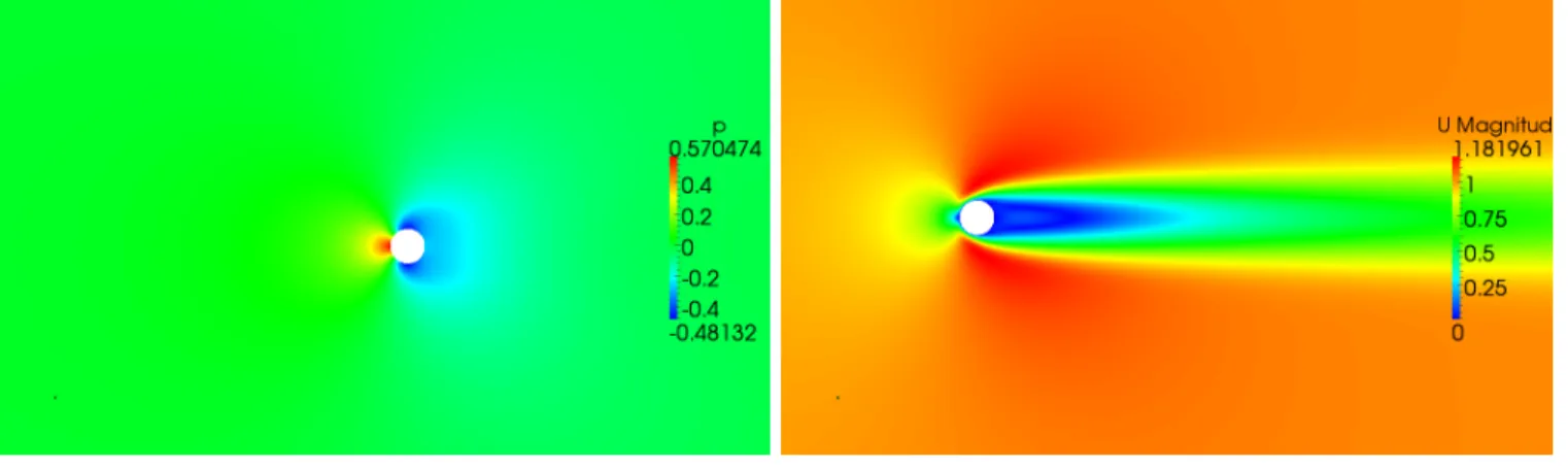
(a)Pressure distribution (b)Velocity distribution

Figure 3.3: Results for pressure and velocity in the circular cylinder case withRe 40

(25)

Figure 3.4: Results for pressure distribution at the circular cylinder wall withRe40

Variable OpenFOAM simulation Simulation A Grove et al Coutencau et al

Separation Angleθ(in degrees) 126.67 126.67 137.2 126.5

Bubble Length L (in diameters) 2.24 2.22 1.54 2.13

CD 1.53 1.58 -

-Table 3.1: Summary results of Re 40 [8]

Conclusion From this test, it can be concluded that the laminar solver of OpenFOAM is accurate for the flow around the circular cylinder as modeled here. The test results are in good agreement with test results as well as with other models.

3.2.3 uRANS simulation at

Re

10

6

The next case studied is a turbulent case. The main point is to compare the results of this simulation with the results found in literature [13] to determine if the set up of the case is correct and to get to know OpenFOAM for turbulent cases.

Set up This case requires a better mesh. If the mesh of the Reynolds 40 case would be used, the results would have been bad if the solution would have converged at all. The mesh has been revised and can be seen in figure 3.5a in complete and zoomed at the cylinder wall in figure 3.5b. The domain size is the same as in the Reynolds 40 case.

(a)Omesh (b)Zoom

Figure 3.5: Mesh used for the circular cylinder case with Re106

(26)

The kinematic viscosityν is set to 1.7e−6m_s2 and the velocityU to 8.5m_s in order to get a Reynolds numberRed of 1e6. The boundary conditions for this case can be found in table 3.2. It should be noted that the velocity is strictly inx1-direction and that the inletOutlet boundary condition prescribes a fixed value if the velocity vector at that cell

points into the domain and a zero gradient boundary condition when the velocity vector is pointed outwards. The ‘calculated’ boundary condition tells the program to calculate the value from the other solved values. The use of wall models can be justified by the fact that they+ _{distribution is between 10 and 40.}

Variable Internal field Edge of domain Wall

U uniform 8.5 inletOutlet 8.5 0

p uniform 0 zero gradient zero gradient

uniform 0.000765 inletOutlet 0.000765 Epsilon wall function

k uniform 0.00375 inletOutlet 0.00375 kqR wall function

νt calculated calculated nutk wall function

Table 3.2: Boundary conditions for the circular cylinder case atRed= 1e6

The time step in this case is 0.00023529s, chosen based on the calculations in the reference paper [13]. The end time was 70.855sand since there will be turbulence, the mean values were taken from 35.2935suntil the end time.

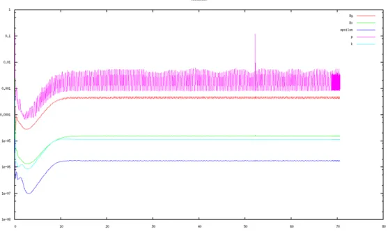
Results The residuals are given in figure 3.6. As can be seen in this figure, the residuals do not go down as in the case of Re40. Instead they move to an equilibrium point and oscillate. These oscillations are caused by the vortex shedding in the unsteady case. Because of the vortex shedding, it is useless to measure the bubble length at a certain time. Instead, all the computations and plots shown here are time averages and averaged from 35 seconds until the end time. The mean pressure and velocity distributions are displayed in figure 3.7 and the pressure coefficient in figure 3.8.

Figure 3.6: Convergence for the uRANS circular cylinder case withRe 1e6

(27)

(a)pressure (b)Velocity

Figure 3.7: Results for pressure and velocity of the circular cylinder case with Re1e6

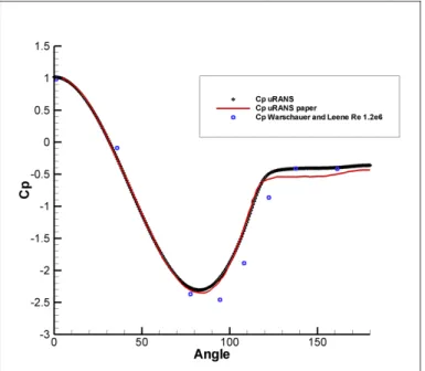
Figure 3.8: Results for pressure distribution at the circular cylinder wall withRe 1e6with the ones of the paper [13]

The Strouhal number is defined as:

St= f L

U (3.1)

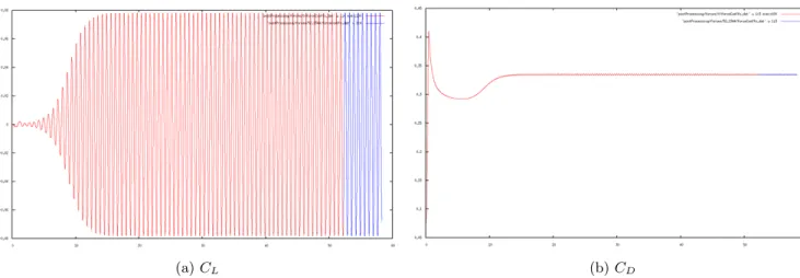
with f being the frequency of the vortex shedding, L the diameter of the circular cylinder and U the freestream velocity. The frequency of the vortex shedding can be determined from the lift or drag coefficient. In order to check the results both methods were used. The results of this case are summarized in table 3.3. It should be noted that the bubble length is the length from the center of the circular cylinder to the end of the bubble.

Variable OpenFOAM

simulation uRANS paper LES paper Exp. Shih et al Exp. others see paper

Separation Angleθ (in degrees) 122.151 - - -

-Bubble Length L (in diameters) 1.41 1.37 1.04 -

-CD 0.33 0.4 0.31 0.24 0.17-0.40

CLmax 0.078 0.12 - -

-St 0.344 0.31 0.35 0.22 0.18-0.50

Table 3.3: Summary results of Re1e6, computations from the paper and experiments [13]

(28)

(a)ux at _Dy = 0.75 (b)ux at _Dy = 1.50

(c)uy at _Dy = 0.75 (d)uy at _Dy = 1.50

Figure 3.9: Results for velocity distribution in the circular cylinder case withRe 1e6 and the results of the paper [13]

(a)CL (b)CD

Figure 3.10: Results for lift and drag coefficient of the circular cylinder case atRe 1e6

atRe 1.2e6. Also when the velocity profiles are studied, it can be seen that a little too much artificial dissipation is added to the system. In next computations, this could be solved by decreasing the cell spacing resulting in a finer grid or by using higher order schemes. The schemes used in the calculations performed in the circular cylinder case are second order. A better result could be found if a third or fourth order scheme is used. However, both increasing the number of cells as well as increasing the order of the schemes will increase the calculation time.

The uRANS computations of the paper need to be inspected carefully, because they do not seem entirely correct. In figures 3.9c and 3.9d it can be clearly seen that the profiles of the paper are not symmetric. Since this is a uRANS simulation, it is expected that these profiles would be symmetric and thus the results should be interpreted with care. The values all seem to be in the right order of magnitude resulting in the conclusion that the model as it is set up here produces some reasonable results.

3.2.4 LES simulation at

Re

10

6

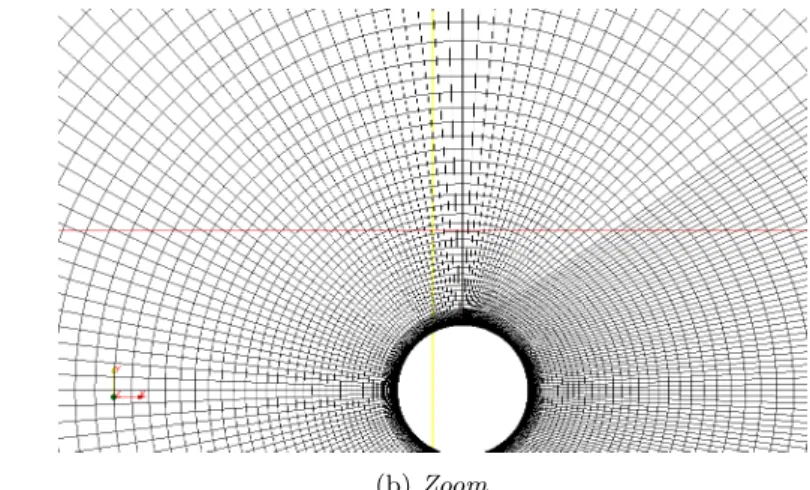
(29)

Set up The major difference in domain between this case and the uRANS case is the domain inz-direction. An LES computation can not be done in two dimensions so the third dimension is extended in comparison to the uRANS computation. The domain inz-direction is set to 4 times the diameter of the circle, as in the reference paper [13], while the rest of the dimensions stay the same. The boundary condition for the front and back patch are now set to cyclic in OpenFOAM which means that will treat these patches as a periodic boundary. The amount of cells used are in respectively radial, circumferential andzdirection: 230 elements, 300 elements and 48 elements. Again, a full view and a detailed view of the mesh can be found in figure 3.11. The cell distribution is uniform inz-direction.

(a)Omesh (b)Zoom

Figure 3.11: Mesh used for the LES circular cylinder case with Re 106

The LES model chosen in this case is the one equation eddy model. This model solves the conservation equation for the turbulent kinetic energyk. This model is used with the van Driest damping function which applies a cube root volume filter. The initial condition for the velocity and pressure is set to the average pressure and velocity field of the uRANS computations. This is done because the main flow field should not change too much between a uRANS and LES case and by applying this initial solution, it is expected to reach convergence faster. The boundary conditions of this setup are displayed in table 3.4.

Variable Internal field Edge of domain Wall

U mapped uRANS 8.5 inletOutlet 8.5 fixed value 0

p mapped uRANS 0 zero gradient zero gradient

k uniform 0.00375 inletOutlet 0.00375 kqR wall function

νSGS uniform 0 calculated calculated

Table 3.4: Boundary conditions for the LES circular cylinder case atRed= 1e6

The time step in this case is set to 0.001secwith a time frame of 0secto 75sec. Again an averaging process is started, this time at 30sec in order to acquire enough data for the statistics.

Results The residuals of this case are given in figure 3.12. Since these residuals are compared to the initial field, the convergence does not automatically go down a lot. The initial field is already the converged solution of the uRANS solution. Especially in a very turbulent LES case, the residuals are usually not the best way of telling if a case converged since the solution fluctuates a lot. Usually another parameter is used in order to see if the case reaches convergence. This other parameter can be a coefficient such as the drag or lift coefficient but also the pressure in a certain point (probe location).

Because the case is three dimensional, the solution, for example the bubble length, also varies with the span. The average bubble shape can be seen in figure 3.13 and as can be seen, it varies with the spatial coordinatez. The average bubble length is calculated to be 0.75D measured from the center of the circular cylinder. The plotted area is the surface at which the mean velocity inx-direction is zero meter per second.

The pressure coefficient is shown in 3.14 and is plotted together with the uRANS results and the experiments of Leendert and Warschauer. The velocity profiles at the different substations can be found in figure 3.15.

The last two figures (figure 3.16a and figure 3.16b) show respectively the lift and drag coefficient.

(30)

Figure 3.12: Convergence for the LES circular cylinder case withRe 1e6

Figure 3.13: Average bubble shape of the circular cylinder LES case forRe 1e6.

Figure 3.14: Results for pressure distribution at the circu-lar cylinder wall with Re 1e6 in LES case with the ones of the paper [13]

(31)

(a)ux at _Dy = 0.75 (b) ux at _Dy = 1.50

(c)uy at _Dy = 0.75 (d)uyat _Dy = 1.50

Figure 3.15: Velocity distribution in the LES circular cylinder case with Re1e6 and the results of the paper [13]

(a)CL (b)CD

Numerical Simulation over a backward facing step with OpenFOAM

University of Twente

Internship at CIRA