Numerical modeling of superconducting YBCO tapes

Twente University

Numerical modeling of

superconducting YBCO

tapes.

A BSc assignment as part of the Applied Physics Bachelor programme

P 1

Table of Contents

1. Introduction ... 2

1.1 Superconducting YBCO tapes ... 2

1.2 Thermal stability & quench behavior of HTS tapes ... 4

1.3 Research outline ... 4

Chapter 2: Modeling of MQE and Vnzp ... 6

2.1 Analytical understanding ... 6

2.1.1 Deriving the heat balance equation (1) ... 7

2.1.2 Cooling term ... 8

2.1.3 Initial power dissipation ... 8

2.1.4 Ohmic power dissipation ... 9

2.2 Normal zone propagation velocity and minimum quench energy ... 10

2.2.1 Normal zone propagation velocity ... 10

2.2.2 Minimum quench energy ... 11

2.3 Numerical Modeling ... 12

2.3.1 Explanation of the time dependent model ... 12

2.3.2 Calculation methods ... 13

Chapter 3: Results of the simulations ... 15

3.1 Effect of number of nodes ... 15

3.2 Effect of Ic scaling relations ... 17

3.3 Effect of the energy pulse ... 20

3.4 Effect of a cooling term ... 22

3.5 Comparing simulations to experimental data ... 23

Discussion and conclusion ... 27

P 2

1. Introduction

1.1 Superconducting YBCO tapes

In 1911, a few years after he succeeded in liquefying helium, H. Kamerlingh Onnes discovered that certain metals such as mercury, lead and tin lose their electric resistance below a certain critical temperature (Tc). This critical temperature is a property of the material. Research with a

superconducting ring has shown that currents do not change in more than 10^5 years. It is even expected that no reduction in field or current is expected in 10^10^10 years. [1]

Then, in 1933, Meissner and Ochsenfeld discovered the now called Meissner effect. They found out that superconductors expel magnetic flux when cooled below the critical temperature. When the magnetic field gets too strong, the superconductor will no longer be able to expel magnetic flux and will return to his normal conducting state. The critical magnetic field (Hc) depends on the

temperature of the superconductor. [1]

The magnetic field also has an effect on the maximum current that can run through a wire. Due to Ampere’s law, there is a certain current where the induced magnetic field is higher than the critical field, thus causing the superconducting properties to be lost. This point is known as the critical current density (Jc) or critical current (Ic) when talking about wires and cables.

These three effects together form a critical surface as seen in Figure 1. As long J, H and T are below this surface, the superconductor is actually superconducting. The exact shape of the critical surface is dependent on the material and the configuration it is in.

http://www.futurescience.com/manual/sc500.html

Figure 1: Critical surface of a superconductor [2]. The darker lines in the right figure indicates the temperature-dependent cricical current density Jc(T,H0) at an applied magnetic field H0.

While initially many superconductors were discovered, the maximum for the critical temperature was stuck at 23K. The big breakthrough was in 1986, when Bednorz and Müller discovered LBCO (Lanthanum Barium Copper Oxide) as a superconductor. While the critical temperature of 35K was impressive, it also opened up a whole new research field revolving around these

P 3

Copper Oxide, Tc = 130K). These new materials are categorized as high temperature superconductor (HTS), while the old materials with a Critical temperature below 30K are low temperature

superconductors (LTS). The big advantage of HTSs is that they can be cooled with liquid nitrogen instead of liquid helium.

While a lot of research has gone into LTS materials, HTS materials are relatively new. Moreover, most research in the HTS field has focused on the high temperature range. For a complete image of HTSs, the low temperature range should also be considered. At a lower temperature the critical currents and critical magnetic fields are higher, allowing for more intense applications.

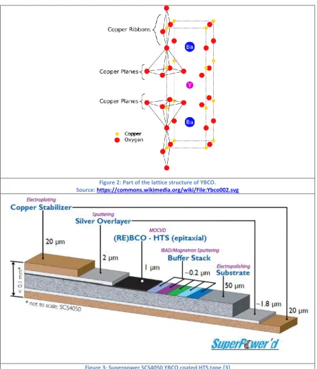
Figure 2: Part of the lattice structure of YBCO. Source: https://commons.wikimedia.org/wiki/File:Ybco002.svg

P 4

This rapport is mainly focused on YBCO superconductors. More about that in paragraph 1.3. YBCO falls in the ‘123’ class superconductors. This class is characterized by its chemical composition: Re1Ba2Cu3O7-x [1]. Here Re stands for rare earth element such as Lanthanum, Neodymium and of course Yttrium. Because these materials are highly anisotropic, its critical field is dependent on the orientation of the field. The critical field is low when it is orientated perpendicular to the copper oxide planes and the highest when parallel to these planes (Figure 2).

Finally in Figure 3 is the full layout of an YBCO coated superconductor. The copper stabilizer is not only useful for increasing the strength of the cable, but also to absorb extra currents without damaging the YBCO layer [3].

1.2 Thermal stability & quench behavior of HTS tapes

In order to apply practical uses to YBCO tapes, it is important to know about its thermal stability. That is, how does the superconductor react when it locally loses its superconductivity. This can happen when a disturbance heats the tape above the critical temperature. When this happens, the normal conducting part will cause ohmic heating. In the case the normal conducting area is small enough, it will cool down and shrink until the entire tape is superconducting again. If the area is too large however, it will expand because the heating is larger than the cooling. When this happens we’re talking about a quench.

If no action is taken, the superconductor will heat up until it burns out. For some magnets it might be sufficient to just cut the power. Larger magnets store a lot more energy in their field. When power is cut for these magnets all this energy still needs to be dumped in the coil. In this case it might be needed to artificially create more normal zones so that the energy dissipates more evenly

throughout the coil, preventing local overheating. The amount of energy needed to create a quench is conveniently called Minimum Quench Energy (MQE). The larger the MQE, the more stable a superconducting magnet is deemed to be.

Another factor, and for this rapport the more important one, is the Normal Zone Propagation Velocity (Vnzp). This velocity is the rate at which the edge between the normal zone and the superconducting zone moves. Not only does a higher Vnzp mean that less artificial normal zones need to be created, it also means that normal zones are easier and faster to detect.

For LTS the quench behavior is extensively studied. The effects of the magnetic field, temperature and current on MQE and Vnzp are well known. This has allowed devices such as MRIs and particle accelerators to exist. For HTS this is not the case. Recent studies have shown quite surprising results regarding the effects of the current and Vnzp [4].

1.3 Research outline

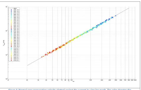
Research done by J. van Nugteren has revealed an unexpected relation between the current and Vnzp. As shown in Figure 4, the normal zone propagation speed scales with the power of 1.491 +/- 0.012 to the current. [4] This rapport is a continuation of that research and will mainly focus on two aspects. Firstly there will be sought for a reason for such a neat power-law. It seems that

temperature and magnetic field have no significant effects on the normal zone propagation speed, while the theoretical understanding suggests it would. For that a simulation will be used to

P 5 Specially, the research questions I investigated were:

 What is the effect of the number of nodes on the simulated normal zone propagation velocity?

 What is the effect of the Ic scaling relations on the simulated normal zone propagation velocity?

 What is the effect of the initial energy pulse on the simulated normal zone propagation velocity?

 What is the effect of a cooling term on the simulated normal zone propagation velocity?

 How does the simulated normal zone propagation velocity compare to the experimental data?

This research is done in parallel with the experimental MSc assignment of Bram Hesselink, who is currently extending the relation between Vnzp and the current to temperatures between 4.2K and 25K.

This rapport will continue in chapter 2 with an explanation of the model. In paragraph 2.1 the analytical understanding will be explained, follow by the numerical model in paragraph 2.2. Then in chapter 3, the results of the simulations will be discussed, as well as a comparison between the simulation and experiments in paragraph 3.4.

P 6

Chapter 2: Modeling of MQE and Vnzp

In this chapter the model used to simulate normal zone propagation will be explained. To start the heat balance equation will be explored in paragraph 2.1. This equation describes how heat generates and flows in a superconductor. It will then be shown how this heat balance equation can be used to find the normal zone propagation velocity and the minimum quench energy. Then in paragraph 2.2 the heat balance equation will be used to introduce the numerical model. For this a string of one-dimensional nodes will be considered. These nodes are used to transform the continuous heat balance equation to a discrete model used for simulation.

2.1 Analytical understanding

The numerical predictions are based on solutions of the heat balance equation schematically

depicted in Figure 5. The one-dimensional form of this equation describes the axial flow, sources and storage of thermal energy in a superconducting wire or tape:

𝐶(𝑇)𝜕𝑇 𝜕𝑡 =

𝜕

𝜕𝑥[𝑘1𝐷(𝑇) 𝜕𝑇

𝜕𝑥] + 𝑃Ω+ 𝑃𝑖+ 𝑃𝑐 (1)

𝐶(𝑇) is the heat capacity in J/Km, 𝑘1𝐷(𝑇) the thermal conductivity in Wm/K and 𝑇, 𝑡 and 𝑥 the temperature in K, time in seconds and one-dimensional position in meter respectively. 𝑃Ω, 𝑃𝑖 and 𝑃𝑐 in W/m are the different sources and sinks of heat in the tape. They are discussed in paragraph 2.1.4, 2.1.3 and 2.1.2, respectively. All units are converted to their one-dimensional form, i.e. expressed per meter length of the tape sample instead of more general volumetric densities. As long as the size of the minimum propagation zone (see paragraph 2.2.2) is larger than the width and thickness of the tape this is no problem. Only when talking about large tapes or multiple tapes in a wire this equation needs to be expanded to the 2-dimensional or even 3-dimensional forms.

P 7

2.1.1 Deriving the heat balance equation (1)

This equation can be derived by taking the first law of thermodynamics (conservation of energy) and applying it to a solid, adiabatic bar. When taking a slice of this bar of length Δ𝑥, the equation

becomes:

𝑞𝑥− 𝑞𝑥+Δ𝑥− 𝑤 =

𝜕𝐸 𝜕𝑡, (2)

with 𝑞 and 𝑤 the heat flowing into and work done by the slice (in W) and 𝐸 its energy. This energy consist solely of internal energy, therefore is given by:

𝐸 = 𝜌𝑀𝐴Δ𝑥 𝑢. (3)

𝑢 is the internal energy density in J/kg, 𝜌𝑀 the mass density of the system and 𝜌𝑀𝐴 Δ𝑥 its mass. Since this system is in gross approximation incompressible, a change in its internal energy is proportional to the change in temperature:

𝑑𝑢 = 𝑐𝑣 𝑑𝑇, (4)

with 𝑐𝑣 the specific heat capacity at constant volume (J/kgK). When combining equations 3 and 4 we get:

𝜕𝐸

𝜕𝑡 = 𝜌𝑀𝑐𝑣𝐴Δ𝑥 𝜕𝑇

𝜕𝑡. (5)

Assuming that all (electrical) work done is converted to heat and not used in deforming the material, the work transfer rate can be written as:

−𝑤 = (𝐴 Δ𝑥)𝑞′, (6)

with 𝑞′ the ohmic heat generated in the solid in W/m^3.

Finally the heat transfer rate is proportional to the temperature difference between the two ends of the slice:

𝑞𝑥 = 𝐶𝑜𝑛𝑠𝑡𝑎𝑛𝑡 ∗ (𝑇𝑥− 𝑇𝑥+Δ𝑥). (7)

Experiments show that this constant is equal to 𝑘3𝐷𝐴/Δ𝑥, with 𝑘3𝐷 an experimental determined “effective” thermal conductivity (by “lumping” together contributions of all materials in the tape in parallel) in W/Km. In the limit of Δ𝑥 → 0, the heat transfer rate becomes:

𝑞𝑥 = −𝑘3𝐷𝐴

𝜕𝑇 𝜕𝑥 (8)

This is the Fourier law of heat conduction. Using this to express the heat conduction out of the slice at 𝑥 + Δ𝑥, it can be rewritten as:

𝑞𝑥+Δ𝑥 = 𝑞𝑥+

𝜕𝑞𝑥

𝜕𝑥 Δ𝑥 = −𝐴 [𝑘3𝐷 𝜕𝑇 𝜕𝑥+

𝜕 𝜕𝑥(𝑘3𝐷

𝜕𝑇

𝜕𝑥) Δ𝑥] (9)

P 8

−𝑘3𝐷𝐴

𝜕𝑇

𝜕𝑥+ 𝐴𝑘3𝐷 𝜕𝑇 𝜕𝑥+

𝜕 𝜕𝑥(𝑘3𝐷

𝜕𝑇

𝜕𝑥) Δ𝑥𝐴 + 𝐴 Δ𝑥 𝑞

′_{= 𝜌}

𝑀𝑐𝑣𝐴Δ𝑥

𝜕𝑇 𝜕𝑡 (10)

Dropping the common factor Δ𝑥 and defining:

{

𝑘1𝐷≡ 𝐴𝑘3𝐷 [

𝑊𝑚 𝐾 ]

𝐶 ≡ 𝐴𝜌𝑀𝑐𝑣 [

𝐽 𝐾𝑚]

𝑃𝑖+ 𝑃Ω+ 𝑃𝑐 ≡ 𝐴𝑞′ [

𝑊 𝑚]

(11)

to go from the general 3-dimensional case to our specific 1-dimensional model, we finally get

𝐶(𝑇)𝜕𝑇 𝜕𝑡 =

𝜕

𝜕𝑥[𝑘1𝐷(𝑇) 𝜕𝑇

𝜕𝑥] + 𝑃Ω+ 𝑃𝑖+ 𝑃𝑐. (1)

2.1.2 Cooling term

In (11) we split the external energy released in the tape (𝐴𝑞′) into three separate sources, 𝑃𝑖, 𝑃Ω and

𝑃𝑐. We first consider 𝑃𝑐, a heat sink by way of lateral cooling to the environment (as opposed to axial heat flow through the tape itself). This cooling term consist of two parts, conductive cooling and radiation. Because the tape is in a vacuum, there is no mass flow to transfer heat. The radiative cooling is given by:

𝑃𝑟𝑎𝑑,2𝐷= 𝐴𝑟𝑎𝑑𝜖𝜎𝑏𝑜𝑙𝑡𝑧∗ (𝑇14− 𝑇24) (12)

With 𝐴𝑟𝑎𝑑 the radiated surface area in square meter, 𝜖 the emissivity and 𝜎𝑏𝑜𝑙𝑡𝑧 the Boltzmann constant at 5.67037321 ∗ 10−8 _W/K4_m2_{. The radiative cooling per meter length (𝑃}

𝑟𝑎𝑑,1𝐷) can be archived by reducing the cooling area (𝐴𝑟𝑎𝑑) to the cooling width (𝑤). Since the tapes used in the experiments are 2-4mm wide, it is set to 4mm. In the most ideal case the emissivity is 1, that of a black body. When the tape is at its 𝑇𝑐, 93K and the environment of the helium bath is 4.2K, the maximal, black body, radiative cooling is:

𝑃𝑟𝑎𝑑,1𝐷= 𝑤𝜖𝜎𝑏𝑜𝑙𝑡𝑧∗ (𝑇14− 𝑇24) = 0.0170

𝑊 𝑚 (13)

A one-dimensional conductive cooling term can be expressed as:

𝑃𝑐𝑜𝑛= ℎ ∗ (𝑇1− 𝑇2), (14)

where ℎ is heat transfer coefficient in W/mK. The real value of h must be determined empirically and will be discussed in paragraph 3.5. We will see that conduction cooling is significantly more

important than the maximum 17mW/m radiation cooling, so for the remainder of this report we will neglect 𝑃𝑟𝑎𝑑 and put:

𝑃𝑐 = −𝑃𝑐𝑜𝑛. (15)

2.1.3 Initial power dissipation

For the initiation of the quench, an additional power term is introduced: 𝑃𝑖. In the experiments described in paragraph 3.5, this “initiator term” is applied as a short (typically < 100 ms) rectangular heat pulse applied in a well-defined location with a quench heater. In ‘real life’ quenches of

P 9

since we’re mostly interested in the steady-state propagation of a normal zone (i.e. the propagation well after the initial transient behavior due to 𝑃𝑖 has ceased to play a major role and the heating term

𝑃Ω drives the growth of the normal zone) and since we want to compare our simulations to experiments, we define this initial power term as:

𝑃𝑖(𝑥, 𝑡) = {

𝛿(𝑥) ∗𝐸𝑝𝑢𝑙𝑠𝑒 𝑡𝑝𝑢𝑙𝑠𝑒

, 0 < 𝑡 ≤ 𝑡𝑝𝑢𝑙𝑠𝑒

0, 𝑡 > 𝑡𝑝𝑢𝑙𝑠𝑒

(16)

The variable 𝐸𝑝𝑢𝑙𝑠𝑒 (in J/m) is used to produce the quench energy and 𝛿(𝑥) is the Kronecker-delta function. The effect of this energy pulse is discussed in detail in paragraph 3.4.

2.1.4 Ohmic power dissipation

The last term is the Ohmic power dissipation. This term is defined as:

𝑃Ω= 𝜌𝐼2. (17)

𝜌 is the “effective” electrical resistivity in Ω/m and 𝐼 the current. Since it has no resistivity, a ‘normal’ functioning superconductor will not heat up. However, if the initial power dissipation rises the temperature of the superconductor above the critical temperature locally, there is no

superconductivity left and Ohmic heating occurs.

Figure 6: Adapted from [4]. Schematic representation of current sharing between the superconductor and the normal matrix. At T = Tsc(B0), the critical current Ic(Tsc,B0) (see Figure 1) becomes equal to the overall current I0. Above this temperature, a part Isc of the current flows in the superconductor, the rest Inc in the matrix (right picture). For computational simplicity, this current sharing regime is often replaced by an abrupt change-over at a transition temperature Tt (left picture)

In reality, the situation is more complex than this simple picture with 𝑃Ω= 0 at 𝑇 < 𝑇𝑐 and 𝑃Ω≠ 0 above 𝑇𝑐. Since the critical current is temperature dependent, there is a region where the

operational current is higher than the critical current, but the T is still smaller than 𝑇𝑐, see Figure 6. The start of this interval is called the “current sharing temperature” (𝑇𝑐𝑠). At this part the current is shared between the superconductor and the normal conductor. Since the current sharing ratio (the amount of current in the normal conducting parts compared to the resistanceless current still carried by the superconductor) depends also on the temperature, a full analytical description is not

P 10

𝑃Ω = {

0 𝑇 < 𝑇𝑡

𝜌𝐼2 _{𝑇 > 𝑇} 𝑡 (18)

The choice of the transition temperature 𝑇𝑡 is somewhat arbitrary, but often 𝑇𝑡 = (𝑇𝑠𝑐+ 𝑇𝑐)/2 is taken (see reference [34] in J. van Nugteren [4]).

2.2 Normal zone propagation velocity and minimum quench energy

Now we have established the heat balance equation we can calculate the rise in temperature as result of the heat generated. This dynamic temperature profile can then be used to derive the normal zone propagation velocity and the minimum quench energy.

2.2.1 Normal zone propagation velocity

The normal zone propagation velocity describes a steady-state situation. This means that the initial power dissipation 𝑃𝑖 is zero since the energy pulse has already passed. For the moment we will assume a fully adiabatic situation, so the cooling term 𝑃𝑐 is also set to zero. This results in the equation:

𝐶(𝑇)𝜕𝑇 𝜕𝑡 =

𝜕 𝜕𝑥[𝑘(𝑇)

𝜕𝑇

𝜕𝑥] + 𝑃Ω (19)

The normal zone propagation velocity is the velocity at which the boundary between the normal conduction zone and the super conducting zone moves. The normal zone propagation velocity can be introduced into the heat balance equation by transforming it from a static x-coordinate system to a z-coordinate system that moves with the normal zone front:

𝑧 = 𝑥 − 𝑉𝑛𝑧𝑝𝑡 (20)

This implies that the boundary between normal- and superconducting is always at 𝑧 = 0. The temperature derivative is now:

𝜕𝑇 𝜕𝑡 =

𝜕𝑇 𝜕𝑧

𝜕𝑧 𝜕𝑡= −

𝜕𝑇

𝜕𝑧∗ 𝑉𝑛𝑧𝑝 (21)

For simplicity, it is then assumed that the temperature in the normal zone is linear, i.e. 𝜕𝑇_𝜕𝑧22= 0, and that the heat capacity and thermal conductivity are constant. Since the boundary between the normal and superconducting zones is now at 𝑧 = 0 and Ohmic power dissipation only occurs in the normal zone, the heat balance equation needs to be split up into a “normal” (𝑧 < 0) and a

“superconducting” (𝑧 > 0) part.

{

𝐶𝑛𝑉𝑛𝑧𝑝

𝜕𝑇𝑛

𝜕𝑧 + 𝜌𝑛𝐼

2_{= 0 𝑧 < 0}

𝐶𝑠𝑉𝑛𝑧𝑝

𝜕𝑇𝑠

𝜕𝑧 + 𝑘𝑠 𝜕𝑇𝑠2

𝜕𝑧2 = 0 𝑧 > 0

(22)

𝑇𝑠(𝑧) is found by solving the differential equation and is:

P 11

In the limit that 𝑧 ≫ 0, 𝛽 = 𝑇𝑠= 𝑇𝑜𝑝, where 𝑇𝑜𝑝 is the operational “background” temperature well away from the normal zone. The constant 𝛾 =𝐶𝑠𝑉_𝑘𝑛𝑧𝑝

𝑠 . The factor 𝛼 can be determined when one

realizes that at 𝑧 = 0 the temperature is equal to the transition temperature (𝑇𝑡):

𝑇𝑠(0) = 𝛼 exp (−

𝐶𝑠𝑉𝑛𝑧𝑝

𝑘𝑠

∗ 0) + 𝑇𝑜𝑝= 𝛼 + 𝑇𝑜𝑝= 𝑇𝑡 (24)

𝛼 = 𝑇𝑡− 𝑇𝑜𝑝 (25)

For the normal zone, the solution of the differential equation is a linear function:

𝑇𝑛(𝑧) = −

𝜌𝑛𝐼2

𝐶𝑛𝑉𝑛𝑧𝑝

𝑧 + 𝑇𝑛(𝑧 = 0)(26)

Again, 𝑇𝑛(𝑧 = 0) is equal to the transition temperature, 𝑇𝑡.

Finally, the heat flow across the normal-to-superconducting boundary should also be continuous:

𝑘𝑛

𝜕𝑇𝑛

𝜕𝑧|𝑧=0

= 𝑘𝑠

𝜕𝑇𝑠

𝜕𝑧|𝑧=0

(27)

Combining (27) with (24) and (26), this results in:

−𝑘𝑛

𝜌𝑛𝐼2

𝐶𝑛𝑉𝑛𝑧𝑝

= −𝑘𝑠(𝑇𝑡− 𝑇𝑜𝑝)

𝐶𝑠𝑉𝑛𝑧𝑝

𝑘𝑠

(28)

Rewriting this for the normal zone propagation velocity finally yields:

𝑉𝑛𝑧𝑝= √

𝑘𝑛𝜌𝑛𝐼2

𝐶𝑛𝐶𝑠(𝑇𝑡− 𝑇𝑜𝑝)

(29)

The product 𝐶𝑛𝐶𝑠 is often combined into a geometric average heat capacity 𝐶𝑜= √𝐶𝑛𝐶𝑠 (30). The resulting equation for the normal zone propagation velocity then becomes:

𝑉𝑛𝑧𝑝=

𝐼 𝐶𝑜√

𝑘𝑛𝜌𝑛

𝑇𝑡− 𝑇𝑜𝑝

(31)

It is worth noting that 𝑘𝑛, 𝜌𝑛 and 𝐶𝑜 are all temperature dependent. To simplify estimates, their values are usually determined at 𝑇̃ =𝑇𝑡+𝑇₂𝑜𝑝. Note that for LTS this is a reasonable approach since the transition temperate is only a few Kelvin above the operating temperature, but for HTS this

difference can be tens of Kelvin.

2.2.2 Minimum quench energy

P 12

cooling. This length is called the minimum propagation length (𝑙𝑚𝑝𝑧). If the normal zone is shorter than this length, cooling is stronger than heating and the normal zone will shrink again. So in order to result in a quench, the initial disturbance needs to create a normal zone that measured equal or larger than the minimum propagation length. This length can be calculated by equating the heating and cooling terms:

𝑙𝑚𝑝𝑧∗ 𝜌𝑛𝐼2= 2𝑘𝑛

𝑇𝑡− 𝑇𝑜𝑝

𝑙𝑚𝑝𝑧

→ 𝑙𝑚𝑝𝑧 = √

2𝑘𝑛(𝑇𝑡− 𝑇𝑜𝑝)

𝜌𝑛𝐼2

(32)

The minimal energy required for a quench is the amount of heat that needs to be released by an initial disturbance to raise the temperature in the entire minimum propagation zone above the transition temperature. This is calculated by the following integral:

𝑀𝑄𝐸 = 𝑙𝑚𝑝𝑧∗ ∫ 𝐶(𝑇)𝑑𝑇 𝑇𝑡

𝑇_𝑜𝑝

(33)

This approach assumes that the heat is evenly distributed across the entire length of the minimum propagation zone. In reality a smaller hotspot will develop and more energy is required to initiate a quench.

2.3 Numerical Modeling

While these analytical expressions allow for a first estimation of the behavior of superconductors, they rely on uncertain variables such as the transition temperature 𝑇𝑡 (see paragraph 2.1.4). Especially in HTS, the transitions from superconducting to normal conducting. In addition, the material properties are not a constant but depend on the temperature. With a numerical model the assumption of a single transition temperature where the material “switches” can be relaxed and the temperature dependence of the material properties can be taken into consideration.

2.3.1 Explanation of the time dependent model

The simulations also use the heat balance equation, however for computer modeling it is impossible to use continuous equations. Therefore the heat equation is transformed to a discrete equation: the system is divided into a series of one-dimensional cells as shown in Figure 7.

Figure 7: The one-dimensional cells that make up the system. From: [4]

Each cell has a thermal capacity and is connected to its neighbours on either side by a thermal resistor. The heat balance equation can be applied to each node as:

𝐶(𝑇𝑖)

d𝑇𝑖

d𝑡 =

𝑘(𝑇𝑖)(2𝑇𝑖− 𝑇𝑖−1− 𝑇𝑖+1)

𝑑𝑥𝑖

+ 𝜌(𝑇𝑖)𝐼𝑛𝑐2 ∗ 𝑑𝑥𝑖+ 𝑃𝑖(𝑥𝑖, 𝑡) + ℎ(𝑇𝑜𝑝− 𝑇𝑖)𝑑𝑥𝑖 (34)

P 13

needs some explaining. Up to now, the heat balance equation was used with a sharp transition temperature. In reality the current will gradually switch from flowing through the superconducting material to flowing through the other parts of the superconducting tape such as the copper layers (see Figure 6). For this, the operating current (𝐼𝑜𝑝) is split between a normal conducting- and a superconducting part such that:

𝐼𝑜𝑝= 𝐼𝑛𝑐+ 𝐼𝑠𝑐 (35)

To find out how much of the operating current runs through the normal conducting material, the following non-linear equation must be solved:

𝐼𝑜𝑝−

𝐸0

𝜌 [ 𝐼𝑠𝑐

𝐼𝑐

]

𝑁

− 𝐼𝑠𝑐= 0 (36)

𝐸0 is the criterion used to determine the critical current, 𝐼𝑐 the temperature- and field dependent critical current (see paragraph 1.1), 𝜌𝑛 the electrical resistivity of the normal conducting parts and 𝑛 the experimental determined n-value of the conductor. This equation expresses the fact that the current paths 𝐼𝑆𝐶 and 𝐼𝑁𝐶 are switched in parallel, generating the same electric field 𝐸 = 𝐼𝑁𝐶𝜌 =

𝐸0( 𝐼𝑆𝐶

𝐼𝑁𝐶)

𝑛

. The last expression is the widely-used power-law field-current relation for a

superconducting material. Also note that 𝜌 is the 1-D equivalent of the electrical resistivity (see paragraph 2.1.4). After the superconducting current has been found, the normal conducting current can easily be calculated. This eliminates the need to choose a fixed transition temperature and replaces it with a function that relies on measureable parameters.

The differential equation is then solved using a so called ‘backward time, centered space’ method. This method used a series of equations such that the temperature profile of the next time step matches that of the previous time step. Conveniently this is exactly what Matlab’s built-in ode15s function does.

2.3.2 Calculation methods

Once the simulation has run, the normal zone propagation velocity, 𝑉𝑛𝑧𝑝, can be calculated

straightforwardly. For each time step the length of the normal zone is determined from the amount of nodes that have a temperature above a chosen threshold value. For each time step the difference in normal zone length can be divided by the length of the step and equated to 𝑉𝑛𝑧𝑝:

𝑉𝑛𝑧𝑝=

1 2

𝑑𝑙𝑛𝑧

𝑑𝑡 (37)

The factor ½ comes from the fact that the normal zone propagates in two directions while the velocity is defined as the speed with which the boundary between the normal and superconducting zone is moving.

P 14

P 15

Chapter 3: Results of the simulations

In this chapter the results of the simulation are discussed. The code itself was originally written by J. van Nugteren as part of his MSc graduation assignment. This chapter is used to explore a bit more in-depth the effects of the different parameters in the simulation. First, in paragraph 3.1, the number of nodes will be discussed in order to find a compromise between accuracy and calculation time. After that the Ic scaling relations will be varied in paragraph 3.2. As J. van Nugteren only studied the quench behaviors at 23K – 47K, the program has no data for lower temperatures. Next the effect of the energy pulse is studied in paragraph 3.3, followed by the effect of cooling to the environment in paragraph 3.4. Finally at the end, the simulation results will be compared to measured data in paragraph 3.5.

3.1 Effect of number of nodes

In the program, the number of nodes can be adjusted to reach a higher precision trading off a longer calculation time. More nodes means that each node has a shorter length. This means the simulation is more like a continuous situation. The drawback is that every node takes up calculation time and in order to simulate in a reasonable time, the number of nodes needs to be limited.

In Figure 8 it is shown that the number of nodes clearly has effect on the “ripple” due to

discretisation. As discussed in 2.3.2, the normal zone propagation velocity is calculated as follows:

0 0.1 0.2 0.3 0.4 0.5 0.6 0

0.05 0.1 0.15 0.2 0.25 0.3 0.35 0.4

#Nodes versus V

nzp ripple

Time [s]

V n

z

p

[

m

/s

]

100 Nodes. Ripple = 0.067 (117%) 250 Nodes. Ripple = 0.028 (59%) 500 Nodes. Ripple = 0.0072 (12%) 750 Nodes. Ripple = 0.0039 (7%) 1000 Nodes. Ripple = 0.0025 (4%) 1500 Nodes. Ripple = 0.0011 (2%) 2500 Nodes. Ripple = 0.0003 (0.5%)

P 16

𝑉(𝑛) =1 2∗

𝑙𝑛𝑧(𝑛 + 1) − 𝑙𝑛𝑧(𝑛) 𝑡(𝑛 + 1) − 𝑡(𝑛) (38)

𝑉𝑛𝑧𝑝(𝑛) =

𝑉(𝑛) + 𝑉(𝑛 − 1) 2 (39)

Here is ‘lnz’ the length of the normal zone, ‘t’ the time and ‘n’ the measuring point. The factor ½ is due to the fact that the normal zone propagates in two directions, but the velocity is calculated in one direction. This way of calculating the velocity has as a downside that the velocity on point ‘n’ falls in between time points ‘n’ and ‘n+1’. To adjust for this the final normal zone propagation velocity is calculated by taking the velocity at points ‘n’ and ‘n-1’ and averaging between them.

Because each node is either normal conducting or superconducting, it is not possible to have a perfectly smooth graph. After each time step a number of nodes transfers from superconducting to normal conducting. In a continuous situation, the edge between the normal zone and

superconducting zone could be anywhere inside one node. In the discrete situation, this edge is always at the end of a node. The result is that every few time steps an extra node is added to the normal zone. The time steps are small (~10−6 _{s), therefore an extra node has significant effects on} the normal zone propagation velocity when conductor length 𝑑𝑥𝑖 corresponding to one node is large. With more and smaller nodes, not only fewer times an extra node is added, but the extra added node also has less of an effect on the velocity.

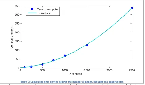
While so far more nodes only have advantages, there is an obvious disadvantage: computing time. In Figure 9 the relation between computing time and the number of nodes is shown. It is clear that this relation is quadratic.

In order to get a proper balance between computing time and accuracy, it is important to look at the resulting normal zone propagation velocity. While using a large number of nodes means the Vnzp at the last time step is a “good” value with a relatively small error, this is not true for the smaller number of nodes. Therefore the average is calculated in two ways. The first one is the easiest one:

Figure 9: Computing time plotted against the number of nodes. Included is a quadratic fit.

0 500 1000 1500 2000 2500

0 50 100 150 200 250 300 350

# of nodes

C

o

m

p

u

ti

n

g

t

im

e

[

s

]

P 17

just calculating the average of the last x time steps. In this example x=15. The second option is taking the average value between the last local maximum and the last local minimum.

#nodes 100 250 500 750 1000 1500 2500

Vnzp (peak to peak) [m/s] 0.0609 0.0569 0.0569 0.0566 0.0567 0.0567 0.0569 Vnzp (last 15 points) [m/s] 0.0633 0.0562 0.0573 0.0566 0.0566 0.0567 0.0568 Table 1: Average of the normal zone propagation velocity.

Table 1 shows the resulting normal zone propagation speed using these two methods. Across the entire line the peak to peak method has better results, especially when using a lower number of nodes. The reason why the first method does not work is because that one is because it is very dependent on where these point lie. If the last point is right on top of a local maximum the average will be larger than when that point is on a local minimum.

The peak to peak method is working so well that even at 250 nodes there is little to no difference between that and the higher number of nodes. If the normal zone propagation velocity at 100 nodes is ignored, the mean value is 0.0568m/s with a standard deviation of 1.1667*10^-4. This means it is safe to choose 500 nodes.

3.2 Effect of Ic scaling relations

As discussed in the intro of paragraph 2.3, one of the advantages of the numerical modeling approach (compared to analytical estimates) is that it can include an accurate description of the current sharing during the superconducting to normal transition (see Figure 6). However, to take full advantage of this description 𝐼𝑐(𝑇, 𝐵) (and 𝑛(𝑇, 𝐵)) must be known. So a proper defined Ic “scaling relation” is important to simulate the normal zone propagation velocity correctly. The term ‘scaling relation’ in this context refers to an accurate analytical expression describing the critical surface (see §1.1, Figure 1). Most research on YBCO superconductors has been focusing on the high temperature range, while for several applications the low temperature range might be more important.

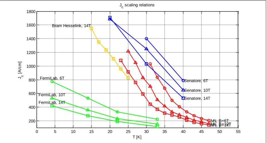
Furthermore it is important that the orientation of the magnetic field is also taken into account. A few Jc-T curves have been plotted in Figure 10.

0 5 10 15 20 25 30 35 40 45 50 55

200 400 600 800 1000 1200 1400 1600 1800

JvN, B=6T JvN, B=10T JvN, B=14T Senatore, 6T

Senatore, 10T

Senatore, 14T Bram Hesselink, 14T

FermiLab, 6T

FermiLab, 10T

FermiLab, 14T

T [K]

J c

[

A

/c

m

]

P 18

Because each tape has a different width, the reported critical currents have been normalized to a critical current density per cm width. SuperPower, the manufacturer of the tape used by Hesselink, reports that each tape has an YBCO layer of 1μm thick.

Researchers at Fermilab [5] investigated the low temperature region of an YBCO tape. Due to their setup, they only measured critical current values in magnetic fields perpendicular to the copper oxide planes. Therefore their values are lower than other data in Figure 10.

The data from Senatore et al. at the University of Geneva shows significantly higher values for the critical current compared to the values measured at the University of Twente by J. van Nugteren and Bram Hesselink. Since is it unclear which tape they used, other than that the manufacturer is

SuperPower, the results can’t be compared one to one.

This is not the case when comparing the data from J. van Nugteren and Bram Hesselink. Even though different widths of tapes were used, the critical current densities are comparable.

Only the Fermilab data extends all the way to 4.2K. For a parallel magnetic field of 14T there is data from 15K upwards. However for lower magnetic fields such as 6T, there is only data from 31K and up. In order to properly simulate a quench at lower temperatures, an 𝐼𝑐(𝐵, 𝑇) relation needs to be created that goes all the way down to 4.2K.

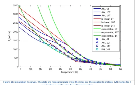
The first one, proposed by J. van Nugteren, expands his measured dataset with some literature data at 4.2K. For the points in between he uses a smooth spline interpolant. This might not be the best option, as it introduces several unexpected (and likely unphysical) inflection points in the 𝐼𝑐(𝑇) dependence, shown in Figure 11.

A second option is suggested by Senatore [6], who uses an exponential relation between the critical current density and the temperature:

𝐽𝑐(𝐵, 𝑇) = 𝐽𝑐(𝐵, 𝑇 = 0) ∗ e− T

T∗ _→𝐽𝑐(𝐵, 𝑇1)

𝐽𝑐(𝐵, 𝑇2)

= 𝑒−𝑇1𝑇−𝑇∗2 ₍₄₀₎

Here T* is a fitting parameter depending on the magnetic field and the specific superconductor used. Jc(B,T=0) is a second fitting parameter.

A downside is that this exponential equation never reaches zero and thus overestimated the Ic at high temperatures. However a critical current density of 6A/cm at 93K won’t have much effect when the operating current density is in the range of 500-1500A/cm. On the low side of the temperature scale the critical current density will go up. The impact of this will be shown later.

The last option is a bilinear fit. The data from Fermilab as well as both datasets from Twente indicate that a relatively accurate description with two linear fits is possible: one for the low temperature and one for the high temperature, with a transition point somewhere around 30-40K, depending on the field.

All three options are shown in Figure 11 for reference.

Figure 10: Temperature dependent Ic values for various Superpower tapes. J. van Nugteren (JvN) [4] used SCS4050 tapes, Bram Hesselink used SCS2050 tapes, the FermiLab used SCS12050 tapes [5] and Senatore [6] did not specify what tape

P 19

Figure 11: Simulation Jc curves. The dots are measured data while the lines are the created Ic profiles. JvN stands for J. van Nugteren and BH stands for Bram Hesselink.

5 10 15 20 25 30 35 40 45 50 55

0 500 1000 1500 2000 2500 3000 3500 Temperature [K] J c [ A /c m ] JvN, 6T JvN, 10T JvN, 14T bi-linear, 6T bi-linear, 10T bi-linear, 14T exponential, 6T exponential, 10T exponential, 14T JvN, 6T JvN, 10T JvN, 14T BH, 14T

0 5 10 15 20 25 30

0.05 0.1 0.15 0.2 0.25 0.3 0.35 Temperature [K] V n z p [ m /s ] Power Law

Data Bram Hesselink, 6T Data Bram Hesselink, 10T Data Bram Hesselink, 14T

I_c scaling JvN, 6T

I_c scaling JvN, 10T

I_c scaling JvN, 14T

bilinear I_c scaling, 6T

bilinear I_c scaling, 10T

bilinear I_c scaling, 14T

exponential I_c scaling, 6T

exponential I_c scaling, 10T

exponential I_c scaling, 14T

P 20

In order to select the “best” curve for the critical current description, the simulated data are briefly compared to the measurements. A more in-depth comparison will be treated in paragraph 3.5. For now only the difference between the simulation and the measurements is discussed and not what these results imply.

Figure 12 and Figure 13 present the simulated data for the normal zone propagation velocity (open symbols) together with measured data from Bram Hesselink (closed symbols), as well as the power law describing the data by J. van Nugteren (solid line). The focus lies on temperatures between 4.2K and 27K. Above these temperatures there is very little difference between the different Ic profiles, thus the profile choice is expected to have very little effects on the Vnzp results.

As a general trend it is visible that all the simulations result in values in-between the measurements from Bram Hesselink and J. van Nugteren. The simulations run with the Ic profile suggested by J. van Nugteren show the biggest spread (i.e. the biggest magnetic field dependence) in the results, even when disregarding the outlier value at 14T, 25K.

The results when using a bilinear Ic profile and exponential Ic profile have a comparable spread. The bilinear profile leads to around 25% higher values for the normal zone propagation velocity than the exponential profile. Because these results are in-between the power law and the results by Bram Hesselink, it is too early to decide if one is better than the other.

3.3 Effect of the energy pulse

The simulation program can also readily adjust the height of the energy pulse that is used to initiate a quench. If this energy pulse is too low, no quench will occur. When the energy pulse is too high, the simulation will abort before the normal zone propagation velocity is stabilized. As mentioned in

P 21

chapter 2, the simulation stops when a node reaches a temperature of 300K. This is always the same node as where the energy pulse is injected. In order to investigate the effect of different pulse height, the same simulation is run multiple times at the same values of magnetic field, temperature and current, while the energy pulse goes from 0.06J up to 0.5J in 11 steps. The results are shown in Figure 14.

Figure 14: Evolution of the normal zone propagation velocity at different values of the initiating energy pulse. B = 14T, T = 35K, I = 100A.

First we consider the 60mJ pulse. This value is below the minimum quench energy and clearly shows the normal zone shrinking again. After the initial energy pulse, the normal zone propagation velocity quickly drops off. At about 0.2 seconds after the pulse, it even becomes negative, indicating that the normal zone retreats.

The 84mJ pulse is close to the minimum quench energy. Vnzp is lower than the higher energy pulses across the entire simulation, although at the end it increases to values near the values induced by the higher energy pulses.

All the other energy levels show similar trends for the Vnzp behavior. The simulations where a lower energy pulse is used run longer than the higher energies and also stabilize earlier, but the end results are very similar. So from the point of view of Vnzp it does not really matter what energy level is chosen since the resulting normal zone propagation velocities are comparable. For the fastest convergence it is useful to simulate near but not below the minimum quench energy, but higher energies can be used to provide a proper indication for the normal zone propagation velocity without spending time to search the minimum quench energy.

0 0.2 0.4 0.6 0.8 1 1.2

-0.05 0 0.05 0.1 0.15 0.2 0.25

time [s]

V n

z

p

[

m

/s

]

Normal zone propagation velocity as funtion of time for various E_pulse

0.06 J

P 22

3.4 Effect of a cooling term

In the real world a fully adiabatic system is not possible. One can approach this limit but some heat will always leak out of the system. Moreover, in the experiments present in the next section, a (load) thermal contact to the environment is made on purpose in order to regulate the starting

temperature 𝑇𝑜𝑝. In order to simulate this, a cooling term (Pc) is introduced in the program. This cooling term can be set to zero to simulate a fully adiabatic system. However in general, a small cooling term is expected. This leads to part of the generated heat being unavailable to heat up the superconducting region out the normal zone, so that Vnzp becomes lower. This effect is more noticeable when the temperature is higher, since the cooling term scales with the temperature gradient. As discussed in chapter 2, the analytical model predicts for the normal zone propagation velocity:

𝑉𝑛𝑧𝑝=

𝐼𝑜𝑝

𝐶 √ 𝜌 𝑘 𝑇𝑡− 𝑇𝑜𝑝

(41)

Here, C, ρ and k stand for the thermal capacity, electrical resistivity and thermal conductivity respectively. While this expression on first sight suggests that a higher operational temperature will result in a higher normal zone propagation velocity, all these parameters are also temperature dependent. So the end result might not be so obvious. Therefore a series of simulations are done with various values for the cooling. The results are shown in Figure 15.

Figure 15: Normal zone propagation velocity as function of temperature for various cooling terms. B=10T and J=375A/cm.

0 5 10 15 20 25 30

0.02 0.025 0.03 0.035 0.04 0.045 0.05 0.055 0.06 0.065 0.07

Temperature [K] V n

z

p

[

m

/s

]

P 23

It is clear that a higher cooling term indeed results in a lower Vnzp. For example, with an

environment temperature of 30K and a cooling term of 1.0W/mK, the same normal zone propagation velocity is found as with an environment temperature of 20K and a cooling term of 0.5W/mK.

Figure 16: Current-dependence of Vnzp assuming h = 0W/mK… Figure 17: … and h = 0.2W/mK. The literature data is the power-law from JvN [4].

Figure 16 and Figure 17 compare the normal zone propagation velocity plotted against the current density for a cooling term of 0 and 2W/mK. The solid line summarizes the power-law is from J. van Nugteren [4]. Note that he used tapes of 4mm width, this rapport is focused on 2mm wide tapes. Therefore his value of 0.4W/mK is not the logical value to use. The simulations confirm this, as a cooling term of 0.2W/mK yields a better correspondence between data and model predictions of tapes of 2mm width.

3.5 Comparing simulations to experimental data

The general conclusion of the experiments by J. van Nugteren in the temperature window 25-50K was that the normal zone propagation velocity mainly depends on the current and not on the magnetic field or the environment temperature. It was suggested that the relation between the normal zone propagation velocity and the current is:

𝑉𝑛𝑧𝑝= 𝑉𝑛𝑧𝑝,0(

𝐼 𝐼0 ) 𝑃 (42) with 𝑉𝑛𝑧𝑝,0

𝐼0𝑃

= 10−4,38

𝑃 = 1,49

Keeping in mind that in that research a 4mm wide tape was used, this can easily be converted to a current density. The research by Bram Hesselink confirms there is a similar relation between Vnzp and current in the 2mm-wide tape he uses, extending the temperature range to 4.2K

Figure 18: Vnzp plotted against temperature. Figure 19 are the same as Figure 12 Figure 13, except that extra data points are removed for visibility. When looking at the data points in Figure 18, the Vnzp is constant and seems not related to the temperature below 15K. At higher temperatures there

150 200 250 300 350 400 450 500 750

0.01 0.02 0.03 0.04 0.05 0.06 0.07 0.08 0.090.1 0.2 J [A/cm] Vn z p [ m /s ]

Relation between Vnzp and Current Density and Temperature, B = 6T,tape width = 2mm

Literauur 31K 35K 39K 43K 47K

150 200 250 300 350 400 450 500 750

0.01 0.02 0.03 0.04 0.05 0.06 0.07 0.08 0.090.1 0.2 J [A/cm] Vn z p [ m /s ]

Relation between Vnzp and Current Density and Temperature, B = 6T,tape width = 2mm

P 24

is a slight rise in Vnzp, from 17% for 6T and 14T up to 26% for 10T, when comparing data points from 4.2K and 29K. While this implies Vnzp depends on the temperature somewhat, the dependency is much less than the analytical relation implies.

P 25

Finally, when looking at the magnetic field, both the simulation as the data points provided by Bram Hesselink show the same pattern. A magnetic field of 6T (circles) result in the lowest values for Vnzp,

Figure 18: Vnzp plotted against temperature.

Figure 19: Vnzp plotted against current density. The thin black lines lie parallel to the thick black line that represents the power law.

0 5 10 15 20 25 30

0.05 0.1 0.15 0.2 0.25 0.3 0.35

Temperature [K]

V n

z

p

[

m

/s

]

Power Law

Data Bram Hesselink, 6T Data Bram Hesselink, 10T Data Bram Hesselink, 14T exponential I_c scaling, 6T exponential I

c scaling, 10T

exponential I_c scaling, 14T

500 550 600 650 700 750 800 850 900 9501000 1250 1500

0.05 0.06 0.07 0.08 0.09 0.1 0.15 0.2 0.25 0.3 0.35

Current Density [A/cm]

V n

z

p

[

m

/s

]

Power Law

Data Bram Hesselink, 6T Data Bram Hesselink, 10T Data Bram Hesselink, 14T exponential I_c scaling, 6T

exponential I_c scaling, 10T

P 26

P 27

Discussion and conclusion

This BSc assignment ran in parallel with an MSc assignment by Bram Hesselink and as a follow up to J. van Nugteren who concluded that the Vnzp in an YBCO superconductor does not depend on the temperature or magnetic field and shows an non-linear relation with the current. A power law was suggested, but only temperatures from 25K and upwards has been tested. Therefore this rapport has tried to confirm this power law dependence for lower temperatures by simulations.

The numerical model used is not flawless. First of all, the discrete nodes cause a jagged line when calculating the normal zone propagation velocity. This can be relieved by using more nodes at the cost that simulations take longer. It is shown when more than 250 nodes are used, the effect of this rippling is avoided by using a smart averaging technique.

Secondly, the current sharing function is very dependent on the critical current. Since there is not sufficient data for Ic at lower temperatures, an Ic extrapolation had to be developed. It was shown that the influence of the precise choice of extrapolating fuction on the predicted normal zone speed is relatively small. The numerical predictions lie between the data from Bram Hesselink and the power law by J. van Nugteren.

Thirdly, the height of the initial energy pulse can be varied. This energy pulse has no effect on the resulting Vnzp values, but it has great effect on the speed of the simulation. An energy pulse with less energy than the minimum quench energy clearly shows that the normal zone gets smaller after the initial pulse. Values for the energy pulse above the MQE all show similar behavior. Although energy levels closer to MQE converge faster, every level results in the same Vnzp.

Finally a cooling term was introduced. This simulated the not perfectly adiabatic environment of a real setup. It depends on the width of the tape used. J. van Nugteren used a 4mm width tape and used a value of 0.4W/Km, while 0.2W/Km was a better fit to the 2mm wide tape used by Bram Hesselink.

After the different aspects of the numerical model were studied, the model predictions could be compared to experimental data from Bram Hesselink and the power law. Both experiments showed

that for an YBCO superconductor Vnzp depends mainly on the current, and the effect of the temperature and magnetic field is smaller. This numerical study can confirm this is the case.

Especially at lower temperatures and higher magnetic fields there is a strong resemblance for this power law. Even at higher temperatures the difference in Vnzp values is at most 27%, much lower than the value the analytical formula suggests.

P 28

Bibliography

[1] M. Tinkham, Introduction to Superconductivity, 2nd ed., USA: McGraw-Hill, Inc., 1996.

[2] Y. Iwasa, Case Studies in Superconducting Magnets, 2nd ed., New York: Springer Science+Business Media, LLC, 2009.

[3] SuperPower Inc., “SuperPower(r) 2G HTS Wire Specifications,” 2014. [Online]. Available: http://www.superpower-inc.com/system/files/SP_2G+Wire+Spec+Sheet_2014_web_v1_0.pdf. [Accessed 14 September 2014].

[4] J. v. Nuchteren, “Normal Zone Propagation in a YBCO Superconducting Tape,” Enschede, 2012. [5] V. Lombardo, “Critical Currents of YBa2Cu3O7-δ Tapes and Bi2Sr2CaCu2Ox Wires at Different

Temperatures and Magnetic Fields,” Batavia, IL, USA, 2010.

[6] C. Senatore, “Overview of the critical surface of industrial CC for EuCARD-2,” University of Geneve, Geneve, 2014.