http://go.warwick.ac.uk/wrap/57617
This thesis is made available online and is protected by original copyright.
Please scroll down to view the document itself.
for
Aperiodic
Dynamical
Systems
Zahir Bishnani
Submitted for the degree of
PhD in Interdisciplinary Mathematics
Mathematics Institute,
University of Warwick
engineering. One is often interested in whether the attracting solutions in these models are robust to perturbations of the equations of motion. This question is extremely important in situations where it is undesirable to have a large response to perturbations for reasons of safety. An especially interesting case occurs when the perturbations are aperiodic and their exact form is unknown. Unfortunately, there is a lack of theory in the literature that deals with this situation. It would be extremely useful to have a practical technique that provides an upper bound on the size of the response for an arbitrary perturbation of given size. Estimates of this form would allow the simple determination of safety criteria that guarantee the response falls within some pre-specified safety limits. An excellent area of application for this technique would be engineering systems. Here one is frequently
faced with the problem of obtaining safety criteria for systems that in operational use are subject to unknown, aperiodic perturbations.
In this thesis I show that such safety criteria are easy to obtain by using the concept of persistence of hyperbolicity. This persistence result is well known in the theory of dynamical systems. The formulation I give is functional analytic in nature and this has the advantage that it is easy to generalise and is especially suited to the problem of unknown, aperiodic perturbations. The proof I give of the persistence theorem provides a technique for obtaining the safety estimates we want and the main part of this thesis is an investigation into how this can be practically done.
The usefulness of the technique is illustrated through two example systems, both of which are forced oscillators. Firstly, I consider the case where the unforced oscillator
Acknowledgements iv
Declaration
V
1 Introduction 1
1.1 Motivation ... 1
1.2 Different approaches to the problem of robustness in aperiodic systems 6 1.2.1 Dynamical systems ... 6
1.2.2 Control theory / Systems theory ... 10
1.2.3 The approach I take ... 10
1.3 Outline of thesis ... 11
2 Hyperbolicity 13 2.0.1 Notation ... 14
2.0.2 Solutions to non-autonomous systems ... 14
2.1 Standard definitions of uniform hyperbolicity ...
15
2.1.1 Equilibria and periodic orbits ... 15
2.1.2 Arbitrary bounded solutions ... 17
2.1.3 Autonomous systems ...
18
2.1.4 Forward and backward contracting subspaces
...
19
2.1.5 Stability type
...
20
2.2 Exponential dichotomy
...
20
2.2.1 Exponential dichotomies on half lines
...
21
2.3 A useful characterisation of hyperbolicity
...
22
2.3.1 Green's functions and the inhomogeneous variational equation 23
2.3.2 The reformulated definition of hyperbolicity
...
27
2.3.3 Splitting index
...
28
2.3.4 Spectral properties of G... 32
2.4 Persistence of hyperbolic solutions ...
35
2.5 More properties of hyperbolicity ...
37
2.5.1 Stability ... 37
2.5.2 Hyperbolic sets ... 38
2.5.3 Structural stability ... 39
3 Safety Criteria 43 3.1 A useful definition of safety criterion ... 43
3.1.1 Interpretation ... 44
3.2 Persistence estimates ... 45
3.2.1 Inverting G... 45
3.2.2 Inverting Cf... 50
3.2.3 Upper bounds for IIxf- xo and estimates of safe perturbations 51
3.3 Example: Additive forcing of equilibria ...
54
3.4 Adapted safety measures ...
55
3.4.1 Adapted norm ...
56
3.4.2 New estimates ... 57
3.4.3 Further refinements ... 59
3.5 Neighbourhood of uniqueness ... 60
3.6 Basins of attraction ... 62
3.6.1 Theory
...
63
3.6.2 Estimates ... 67
4 Generalisations
69
4.1 Discrete time systems ... .... 694.1.1 Hyperbolicity
...
....
69
4.1.2 Persistence of hyperbolic solutions
...
....
70
4.1.3 Hyperbolic sets ...
....
70
4.1.4 Estimates
...
....
71
4.2 Discontinuous perturbation ... .... 71
4.2.1 Some useful functional analysis
...
....
72
4.2.2 Generalisation of hyperbolicity
...
....
79
4.2.3 Persistence theorem
...
....
86
4.3 Further generalisations
...
....
86
4.3.1 Finite time estimates
...
...
87
4.3.3 Autonomous systems and normally hyperbolic manifolds ..
88
5 Applications 90 5.1 Forced damped oscillators ... 90
5.1.1 Equations of motion ... 90
5.1.2 Ship stability and the `escape equation' ... 91
5.1.3 Persistence estimates ... 95
5.1.4 Adapted estimates ... 110
5.1.5 Parametrically forced oscillator ...
113
5.2 Phase-locked loops ... 115
5.2.1 Robustness of phase-locked loops ... 116
5.2.2 Persistence estimates ... 117
5.2.3 Example: External forcing with amplitude and frequency modulation ... 118
6 Concluding Remarks 119 6.1 Summary ... 119
6.2 Limitations of the approach ... 120
6.3 Directions for further research ... 121
A Implicit
Function Theorem
123me to this fascinating area of research and has constantly been a source of enthusiasm, advice and brilliant ideas. He always made time for me and made sure my work progressed
in the right directions. I am privileged to have had such an excellent supervisor.
I was fortunate enough to have spent a year at the Laboratoire de Topologie, Universite de Bourgogne and this was an extremely enjoyable experience. I would like to thank the
staff there for making me feel so welcome and the two guys I shared an office with, Daniel Panazzollo and Gregory Mendausse, for being great company throughout the year.
I would also like to thank the Department of Applied Mathematics and Theoretical Physics, University of Cambridge for hosting me during my final two years of research. While there, I benefitted enormously from discussions with my colleagues in the Nonlin- ear Centre. Jacques-Alexandre Sepulchre introduced me to some crucial mathematical techniques and made useful comments concerning the presentation of my thesis. Swan
Kim was always enthusiastic about my work and gave me excellent advice on how to be a more effective researcher. Mark Johnston and Sinisa Slijepcevic were always around to bounce ideas off and frequently returned them with added value. Allan McRobie from the Engineering Department also made useful comments about my work.
There are a few other people I would like to thank for helpful discussions. I benefitted from numerous conversations with Mark Muldoon whilst at Warwick. Also, Jack Hale
and Steve Montgomery-Smith were extremely enthusiastic when I met them during the "Finite to Infinite Dimensional Dynamical Systems" programme at the Newton Institute.
My primary source of funding has been a studentship from EPSRC. Financial assis- tance has also been provided by awards from Trinity College and the ERASMUS scheme. I am extremely grateful for the support of all my friends who have kept in contact
with me during my research and provided me with an active life outside of mathematics. Without this I would surely have gone crazy. I especially appreciate the efforts of the following people: Andrew Finch, Jason Annadani, Javier Fuente, Catherine Casson, Tom Ash, Katherine Pierce, Shoaib Alam, Alistair Caunt, Fiz, Sylvia, Jim, Rudeboy Randall, the `Rider, and last but not least MC Zebra.
Finally, I am eternally grateful to my parents for being so supportive and encouraging and who have made it all worthwhile by being so proud of my academic achievements.
All the work described in this thesis is believed to be original, except where explicit reference is made to other sources. This thesis is the result of my own work and includes nothing which is the outcome of work doen in collaboration. No part of this thesis has been, or is being, submitted for any degree other than that of Doctor
of Philosophy at the University of Warwick.
Introduction
1.1
Motivation
One of the most common and successful ways of modelling interesting phenom- ena in science is to use dynamical systems. There is a great history to this area of mathematics much of which originates from the use of differential equations in physics. Differential equations arise quite naturally, for example, as a result of applying Newton's laws of motion to physical bodies. For a long time there was an emphasis on searching for exact solutions to differential equations and although this produced a useful theory for certain classes of linear equations, it proved to be
an unsuccessful approach for most nonlinear equations. Starting with Poincare's discovery in the late nineteenth century of non-integrability in celestial mechanical models, it became clear that for typical nonlinear systems, including those with only a few degrees of freedom, exact solutions could not be found. Thus the emphasis shifted to the question of qualitative behaviour in dynamical systems. Poincare himself developed much of this qualitative theory applying many more geometric ideas than previously used. This approach was continued by Birkhoff, Liapunov and many others in the first half of this century and from these important early works sprang an exciting branch of mathematics. In the Sixties many of the geometrical ideas of Poincare and Birkhoff were formalised and developed further by, amongst others, Smale, Bowen and Arnold. I refer to this qualitative theory of nonlinear systems as traditional dynamical systems theory. The books by Guckenheimer & Holmes [14], Katok [20] and Wiggins [57], for example, are good introductory works. Since then nonlinear dynamics has exploded into a very significant area of research not only in mathematics but also in many other areas of science and engineering.
Reasons for this include the massive increase in the use of computers and numeri- cal simulation techniques in the applications and also the popularisation of `chaos
theory' in recent years.
The usual starting point is a dynamical system coming from a mapping or from an ordinary differential equation (ODE). I concentrate on ODE's in this thesis as they are of greater interest in the applications. It is much more common to start with a continuous-time system when modelling real world phenomena. However, on some occasions a discrete-time model is actually more natural. For example, in many ecological situations, especially where breeding is seasonal, one need only consider the population of a given species once per generation. More examples can be found in economics, where decisions or transactions are often made at discrete times like weekly or quarterly. Mappings are also important because they can appear naturally in the analysis or the numerical simulation of continuous-time systems. Most of the work in this thesis has a straightforward extension to mappings and I give a brief sketch of how this works.
There is also great interest in the use of partial differential equations (PDE's) which are systems with more than one independent variable. However, the theory for PDE's is somewhat different in nature and does not usually come under the umbrella of dynamical systems theory. I concentrate on systems where time is the only independent variable although, in principle, some of the results obtained here could be generalised to PDE's. Also of interest in many applications are models with some stochastic element in the equations of motion. Again this theory is different
in nature and I do not deal with it in this thesis.
The main issue I address is the robustness of dynamical behaviour in aperiodic, nonlinear ODE's. The principle motivation for treating this problem is the need for rigourous and effective safety criteria in physical systems where robustness to unknown perturbations is required. This is a largely undeveloped area of dynamical systems theory and there are two main reasons for this.
Firstly, the traditional theory of dynamical systems usually starts with au-
tonomous systems, that is, systems with no explicit time-dependence in the equa-
tions of motion. Much of the theory that follows from this starting point can be
extended to non-autonomous systems but there are some important differences es-
pecially when the system is aperiodic.
cally conjugate solutions in `close' dynamical systems, but the standard proofs do
not naturally give estimates of the degree of closeness
required.
The approach I take addresses both of these problems. I have presented an extension of some the well developed theory of autonomous systems to the non- autonomous case, taking care to make as few assumptions as possible about the time-dependence. The main purpose in doing this is to enable one to provide useful quantitative information relevant to the problems of robustness and stability.
An example of the type of application I have in mind is the problem of ship stability which I treat in some detail in chapter 5. The usual dynamical model is a simple forced oscillator system known as the escape equation or capsize equation,
The external forcing comes from wind and waves. Typically this external forcing is assumed to be periodic. In [51,52,28,29] for example, Thompson and colleagues give some very interesting results regarding the dynamical behaviour of solutions under increasing amplitudes of sinusoidal excitation. It is fully recognised in these works that steady-state analysis and linear approximation techniques are insufficient in highly non-linear situations and thus cannot account for the real danger to stabil- ity facing a ship at sea. The conclusion is that one needs to account for dynamical behaviour under perturbation and protect against transient capsize. Thompson and colleagues have proposed new safety measures such as an index of capsizability. The methods used are geometrical or topological in nature and rely heavily on the fact that for periodic systems one can reduce to a Poincare mapping and then perform a good phase-space analysis based on numerical simulation. Doing this, one finds a variety of phenomena including saddle-nodes, period doubling cascades, indeter- minate jumps, fractal basin boundaries and homoclinic tangles. The qualitative behaviour of such low-dimensional systems is of course of considerable mathemati- cal interest. ' However, the issue that is of fundamental importance in this situation is the practical determination of criteria which guarantee that the ship does not capsize or undergo large motions. When there is no external excitation, there is an asymptotically stable equilibrium where the ship is vertical. When there is forcing, we would like to know the form of the response and more importantly, an upper bound on it's size. In reality of course, the external forces affecting a ship at sea are aperiodic and largely unknown in form. It is not clear at, this stage whether the bifurcation scenario when the forcing is `nearly' periodic resembles closely the peri- odic case as detailed in [51,52]. Johnson's paper [17], for example, suggests that it
does not although there is very little known in general about aperiodic bifurcations. More importantly for present purposes, there seems to be no theory so far in the literature which provides good upper bounds for the size of the response to a given
size of forcing without overly restricting the type of forcing considered.
The ship stability problem is one which has had considerable attention in recent years. It is however, only one of the many dynamical systems used in engineering applications where robustness is an important issue. For example, McR. obie [28] gives many more examples from marine technology. The area of electrical and electronic engineering is also rich with applications of ODE's. Two interesting ones in this area are the swing equation in power generation and phase-locked loops in analogue to digital conversion [21]. Of course, in addition to engineering, there are numerous other fields in which one finds questions of robustness and stability in relation to dynamical system models. For example, many biological systems are modelled by ODE's, and one is often concerned whether the behaviour of the models is robust to external perturbations. Murray [31] is a good introduction to this area. In analysing the periodically forced, escape equation for ship stability there is the advantage that one is essentially dealing with a two dimensional system. Thus geometrical and topological methods are reasonably well suited. However, it is not clear how easily the techniques generalise to higher dimensional systems.
The general problem of robustness I am interested in can be stated as follows.
Consider the first-order non-autonomous system
x=
where xE 1l . Note that one can always write an 01-order system in this way so
it is quite a general form. Suppose that x= fo(x, t) is the unperturbed system and
has an attracting solution xo(t), for example, an equilibrium or periodic orbit. If
f is thought of as a perturbation of fo, the problem is to determine the form of
the response of the system and in particular whether it satisfies some pre-defined
safety conditions, for example belonging to some pre-specified region of phase-space.
When xo satisfies a condition called uniform hyperbolicity, it will be shown that,
for f-
fo small enough, there is a uniformly close attracting solution xf(t) of the
perturbed system. One also has this persistence property for unstable uniformly
hyperbolic solutions and in fact for uniformly hyperbolic invariant sets.
It is a standard approach to the problem of robustness to assume that the perturbation is periodic. For example, for external driving it is often assumed
that excitation is sinusoidal. Doing this makes it relatively simple to determine the response to various amplitudes and frequencies of driving force. One obtains a frequency-response curve this way and this is an extremely important measure which is commonly found in the engineering literature.
There are a number of reasons for assuming periodicity.
" It is sometimes a realistic assumption that the system will be exposed to periodic or roughly periodic external perturbation.
" It is a simplifying procedure and the analysis can become more tractable. There is already a great deal of literature on the subject of periodic systems and the methods are well proven.
9 It is relatively easy to do numerical simulations.
. In linear systems the optimal, `resonant' driving forces are periodic.
However there are also a number of reasons why I believe this approach can be unsatisfactory.
" Safety criteria based on periodic perturbation are often used in cases when
one really does expect perturbations to be aperiodic. These criteria cannot
then be rigourous.
" In this thesis I present an analysis which is reasonably easy to perform and which does not require periodicity. This shows that assuming periodicity is
not the only tractable approach.
" In numerical simulations of periodic systems, one often discovers a wealth of interesting dynamical behaviour. Whether this behaviour manifests itself in the real systems being modelled is a fairly open question. The analysis in this thesis could be used to answer this question in the case of non-bifurcation
behaviour which is an important first step.
" For typical nonlinear systems, the optimal, resonant driving forces are not
periodic.
present here are one way of doing this and follow naturally from a dynamical systems perspective although I present a different formulation to much of the traditional dynamical systems literature.
Another safety estimate of obvious importance is a lower bound for the size of the basin of attraction for asymptotically stable solutions. Here the motivation is safety with respect to perturbations in initial condition. This is often done numerically, for example [44], but I would like to highlight some situations for which the standard methods are not satisfactory and for which the analytic approach I develop could
prove more fruitful.
" When there is high dimensional or infinite dimensional phase space, numerics could be computationally expensive and thus prohibitive. I develop a tech- nique which works in arbitrarily large spaces and which can give estimates that are uniform in system size.
" High dimensional parameter space. Again, computationally this is problem-
atic so analytic estimates could be extremely useful.
" Aperiodic systems often require computation over long time scales. My ap-
proach can often give estimates which are uniform in time.
" When there are `unknown' perturbations one cannot numerically investigate the basins of attraction of the response. With the methodology I present here there is a natural way of estimating the basin size of perturbed solutions even
though they are essentially unknown.
1.2
Different
approaches to the problem of ro-
bustness in aperiodic systems
Here I summarise some approaches that can been be found in the literature which in some way are relevant to the problem of robustness of aperiodic systems.
1.2.1
Dynamical
systems
The concept which is of fundamental importance to almost every dynamical systems approach to the robustness problem is that of uniform hyperbolicity. Ro- bustness to perturbations is a natural consequence of uniformly hyperbolic solutions or uniformly hyperbolic invariant sets. It is also usually the case that a lack of uni- form hyperbolicity implies some form of non-robustness so the concepts are to some extent equivalent. In the next chapter I treat this theory in some detail.
It might be expected that from the ideas contained in the standard proofs of robustness and stability in dynamical systems theory there are ways of obtaining quantitative information like estimates of response size. However this particular issue is very rarely addressed.
Time-dependent
structural
stability
One of the first results from the dynamics community concerning robustness in aperiodic systems is the concept of time-dependent structural stability.
An autonomous dynamical system is said to be structurally stable if every `nearby' system has a qualitatively similar phase portrait. Greater details of this concept are given in the following chapter. The concept of time-dependent struc- tural stability is a generalisation that allows non-autonomous perturbations.
A diffeomorphism f is called time-dependent structurally stable if there is some neighbourhood U of f in the space of diffeomorphisms such that for any ne 7G, fn is topologically conjugate to the composition of an arbitrary sequence of diffeo- morphisms fo 0 fl 0. ""of,,, each of which is picked from U. Since time-dependent perturbations of f can be thought of as a sequence such as this, one could derive use- ful safety criteria by estimating the size of the allowable neighbourhood, although
to my knowledge this has not been done.
This concept has been introduced by Franks in [12] where he shows that uni-
formly hyperbolic systems are time-dependent structurally stable.
Shadowing
Another result which is relevant to aperiodic perturbations of autonomous sys-
tems is the shadowing lemma of Bowen and Anosov. More details of the discrete-
time version can be found in Lanford [22], but here is the basic idea.
Roughly speaking, given a reference system, a pseudo-orbit is an orbit obtained
by allowing any `small enough' time-dependent perturbation. "
The shadowing property is said to hold if, for every small enough pseudo-orbit there is a uniformly close true orbit. This true orbit is called a shadowing orbit. The shadowing lemma says that any uniformly hyperbolic invariant set has the
shadowing property.
One can use the shadowing property to show robustness of a solution to ape- riodic perturbations in the following way. From the sketch definition above, the unperturbed solution is a pseudo-orbit of the perturbed system. Thus if the shad- owing property holds, there is a true orbit of the perturbed system uniformly-close. Thus the unperturbed solution can be seen to be robust. What is required for this idea to be of use in the problem of safety criteria is a clean proof which gives good estimates. I believe this can be obtained most satisfactorily using the framework I present in this thesis although I attack the problem of robustness more directly. For an idea of the use of shadowing estimates see Sauer & Yorke [43], or Coomes, Kocak
& Palmer [33]. These papers treat the problem of determining global error estimates for numerical integration of ODE's by using a functional analytic characterisation
of hyperbolicity.
Skew-Product
Systems
An idea in fairly common use is to consider a non-autonomous system as being the product of a forced system and a forcing system with the property that the forcing dynamics are independent of the forced dynamics.
Definition
1.1 A skew-product system is a dynamical system of the form
x= fl (x, y) (1.1)
f2 (Y) (1.2)
(1.1) is the forced dynamics and (1.2) is the forcing dynamics.
The most simple way to treat the differential equation : i; =f (x, t) as a skew-
product system
is to consider the modified system
x= (x, y) (1.3)
y=1 (1.4)
An extension of this approach is to consider the following modified system.
= F(x, y) (1.5)
y= 9(y) (1.6)
Here the time dependence has been treated as the `output' of some forcing dynamical system on a compact phase-space Y. This is useful if the forcing dynamics are known to come from a low-dimensional autonomous system but this is not often the case for general perturbations of physical systems. For example, the unknown perturbations affecting a building or a ship could only realistically be assumed to
come from a high-dimensional or stochastic dynamical system.
However, given this assumption, much can be said about such systems including interesting things about robustness and stability of solutions. Again, the important condition for robustness is hyperbolicity. For some theory in this vein see Stark
[47]. I do not consider this situation since I am interested in allowing as general a time-dependence in the system as possible.
A second and perhaps more useful way of using the skew-product approach is to first consider the linearisation of i=f (x, t) about some known solution :z0. This gives us a linear non-autonomous equation
ý= Df,;
o(t),
tý
(i. 7)
For reasons I will discuss in detail in the following chapter, study of this equation can tell us most of the essential things about robustness and stability of EO.
We can treat (1.7) as a skew-product system by considering the matrix-valued function Dfxo(t), t as the forcing dynamic and ý as the forced dynamic. This is essentially the approach taken by Sacker & Sell in a series of papers [38,39,40,41, 42].
The approach is most effective when the asymptotic behaviour of Df,; o(t, ), t is known since in that case one only needs to consider the `limit points' of Df; r0(t), t. When these are not known the situation is more complicated.
1.2.2
Control theory / Systems theory
Another approach to the problem of deriving safety criteria can be obtained from a control theoretic viewpoint. The idea is to treat the perturbation or external forcing as a control variable. Then the objective is to induce the largest response for a given size of forcing. Thus the relevant optimal control problem is to search for a worst case scenario. Once the optimal perturbation is found, it is then easy to obtain the maximum response numerically.
For additive forcing it is well known that, for a given maximum amplitude, the control strategy which induces the largest Ck-norm response is of bang-bang type. That is, the control always takes the maximum amplitude but switches direction from time to time. Typically this has a non-trivial switching locus so apart from a few exceptional cases it cannot be found explicitly.
If we are interested in (preventing) responses which have large `energy gains', then some answers are given in the work of Hubler, (see for example [5,56]), who has formulated the principle of the dynamical key. This work seeks to bound the energy gain of a system in terms of the L2-norm of the external forcing function. One can formulate this as a variational problem and this way find the optimal control strategy. The surprising result is that the optimal forcing is just the time- reflected dynamics of the unperturbed system. Since this can be readily determined numerically, one can easily find an upper-bound for the energy gain of the response. This result appears to rely on the self-adjoint nature of the problem when defined on L2 functions and may not generalise easily to more typical cases.
1.2.3
The approach I take
In this thesis, I develop a functional analytic approach to aperiodic systems and suggest that it is the most useful and general one to take. Although it is not a new idea to characterise dynamical systems using functional analysis it is certainly less common than the traditional geometric viewpoint and in consequence is rarely used in applications.
1.3
Outline
of thesis
As I have mentioned, it is a well known result in traditional dynamical systems theory that a solution which is `hyperbolic' is robust to perturbations. It is also true to say that robustness, in the sense of unique nearby continuation, is only present when there is uniform hyperbolicity. This idea extends to uniformly hyperbolic invariant sets, an example of which is the Smale horseshoe. Although the theory of uniformly hyperbolic sets is one of the cornerstones of dynamical systems theory, a formulation of the theory which naturally incorporates aperiodic systems is not easily found in the literature. In chapter 2, I present an extension of the standard theory to aperiodic systems. In particular, I present a characterisation based on lin- ear operators acting on Banach spaces and argue that it is a unified approach which generalises easily and is especially suited to the problem of obtaining safety criteria when there are arbitrary, bounded perturbations. There are two very important results in this chapter. Firstly, I show the equivalence between hyperbolicity of a solution and invertibility of a certain linear operator G. Secondly, I give a theorem which states that hyperbolic solutions persist under small enough perturbations of the vector field. This by proved by using the implicit function theorem and the invertibility characterisation of hyperbolicity. All of the results in chapter 2 can be deduced or found in the current literature and full references are given. However, a suitable, unified exposition of the theory is not available in the literature.
In chapter 3, I tackle the problem of obtaining good safety criteria. The method I use is based on the persistence of hyperbolicity. The crucial element of this method is estimating the response to perturbations by finding an upperbound for the norm of an associated linear operator. This can be practically achieved in a variety of
circumstances and I discuss how one should do this.
An important extension of the method is given in the section on adapted es-
timates. It is clear that some perturbations will be more harmful than others in
terms of the response they
induce. Thus the region of `safe' perturbations is very
far from being shaped like a ball in the space of perturbations. By adapting the
norm one uses
in this space one can take account of this effect to some extent. This
gives us a better estimate of
the shape of the region of safe perturbations and thus
more effective safety criteria.
analytically using the persistence of hyperbolicity property. This is especially use- ful for high dimensional systems since the results are uniform in system size. In
particular the method can be used to find basin of attraction estimates for solutions of perturbed systems even when the precise form of the perturbation is unknown.
In chapter 4, I consider generalisations of the theory. Firstly, there is the impor- tant area of discrete-time systems. Although less common in applications, they are still a very important part of dynamical systems theory and I show that the results for continuous-time systems immediately generalise to the discrete-time case.
The second important generalisation is to systems with discontinuous perturba- tions. For example, external forcing which is bounded in Lu-norm or even impulses. Although in previous chapters I have dealt with spaces of functions and vector-fields that are continuous with respect to time, one can extend the theory to more general function spaces. To do this I present the relevant ideas from functional analysis, in particular, theory concerning the Lp spaces, the Sobolev spaces and spaces of distributions. Then a generalisation of persistence of hyperbolicity theorem is given and used to obtain safety criteria.
In chapter 5, I present some applications of the theory. Firstly I consider ro- bustness and stability in a simple aperiodically forced oscillator system. This has particular relevance to the problem of ship stability and more generally escape phe- nomena. I show in detail how one can obtain safety criteria and I compare these to results from numerical simulations.
A second application is the robustness of `phase locking' in an aperiodically
forced oscillator. I show that the concept of phase-locking makes sense for aperiodic
systems and
derive in detail some lower bounds on the size of perturbation required
to break the phase-locking effect. An interesting technique I develop in this chapter
is the use of a re-parametrisation of time. This is neccessary in order to incorporate
frequency modulation into the general framework.
Hyp erb olicity
A good introduction to the theory of uniformly hyperbolic invariant sets is given by Lanford [22]. Like most of the approaches to this subject he treats only au- tonomous, discrete-time dynamical systems. However, it is one of the few exposi- tions which does not rely solely on a geometric approach. More details, including the theory for continuous-time systems, can be found in the books by Robinson [36]
and Shub [46].
A good formulation of the theory which naturally incorporates aperiodic systems is not available in the literature so I present here in detail the key definitions and theorems. I first give non-autonomous versions of the standard definitions and properties of hyperbolicity. Then I consider a characterisation of hyperbolicity based on operators acting on Banach spaces and show it is a unified approach to the theory and allows for clean proofs and greater generality.
Some early examples of a related approach can be found in the theory of expo-
nential
dichotomy for linear time-varying ODE's. This was developed by Massera
& Schaffer [26], Coppel [7], Daleckii & Krein [9] and Sacker & Sell [39,40,41,42],
in the 60's and 70's although it stems from the ideas of Perron and Bohl in the
early part of the century.
Later in this chapter I present the relevant aspects of this
theory.
Mather [27], has also given a functional analytic characterisation of hyperbolic-
ity for autonomous dynamical systems. Another example can be found in Aubry, MacKay & Baesens [2], MacKay [24] and Sepulchre & MacKay [45], where they have successfully used essentially the same characterisation of hyperbolicity to in- vestigate the dynamics of networks of coupled units. Networks are discrete-space dynamical systems with high or infinite dimensional phase space so are naturally suited to a functional analytic approach.
2.0.1
Notation
Let X be an arbitrary Banach space, with the norm 11. For an interval ZC IR and kEN, let CIc(1, X) denote the Banach space of k-times continuously differ- entiable functions x: I -+ X which are bounded and have k bounded derivatives. This is given the standard Ck norm
Ixllck = max{ IIxII., IIr(k)H }
where II x1Ioo = suptEZ I x(t)I "
For convenience, I abbreviate Ct` (R, Rn) to Ck as it will be the primary space of interest. Also, I abbreviate Ck (1R+, R) to C+ and CIc (R- , IE8" ) to Ck .
In applications one is often interested in obtaining uniform bounds for the norm of the state variable and its derivatives. This is why the CC norm is the most natural choice. In principle one could use a different norm on Ck as long as it remains complete. For example, one could use the weighted norm
HHxllck = max{ wo llxlL, Wi Wk 11.1. (k)1 ". }
with an arbitrary choice of weights, wi E 1[8+ \ {0}. In particular, if one is more interested in j jx jj than the norm of its derivatives then a good choice would be to make wi/wo «1 for i 0.
Denote by BL', the space of bounded linear maps A: R7 --* E V. This is just
the space of nxn
matrices. With the linear operator norm
Al = IIAIIRn-+Rn
= sup
Ivl=1
IAvi
this is a Banach space.
For an element xo in the Banach space X and µE Ili, let Bx (µ, xo) be the size
µ open-ball
in X centred on x0. Formally
Bx(µ, xo) _ {xEX I IIX
- zoll<Et}
Let the symbol D denote
aý
and the symbol ' denote A.
2.0.2
Solutions to non-autonomous
systems
Consider the non-autonomous dynamical system
x=
.f
(X, t)
(2.1)
.f is Cl with respect to x for fixed t, and the Jacobian satisfies l Df1., tl < -Al with M independent of t
"f is CO with respect to t for fixed x.
The theory generalises to dynamical systems defined on differentiable manifolds
but for notational and presentational convenience I just consider systems defined
on ]fin .
Definition 2.1 A (bounded) solution of (2.1), is a function xc C1, such that x(t) satisfies (2.1) for all tER.
Note that I do not include an initial condition but instead consider any solution bounded for all time. One could treat initial value problems by considering solutions on the positive half-line only. I treat this case to some extent in a later chapter where estimates of basins of attraction are obtained, although, it could also be useful to extend all the hyperbolicity theory in this chapter to initial value problems and solutions on half-lines. I give some ideas of how this can be (lone later.
2.1
Standard definitions of uniform hyperbolicity
Definition 2.2 The linearisation, or variational equation of x=f (x, t) about a bounded solution x0, is defined by
= Dfýoct>,
t e
(2.2)Clearly, Df fo(t), t is continuous and uniformly bounded. Let Xo(s) denote the principal matrix solution of (2.2). That is, the matrix solution for which Xo(0) = I. Define the evolution operators by Xt(s) = Xo(s)X0 1(t). These are matrix solutions of (2.2) which satisfy Xt(t) = I. They are also known as fundamental solutions.
2.1.1
Equilibria
and periodic orbits
The most simple solution one can consider is an equilibrium. The following are
standard definitions.
Definition 2.3 An equilibrium solution xa, of an autonomous system x=f (x) is hyperbolic if the Jacobian Dfxo, has no purely imaginary eigenvalues. It is linearly attracting if each eigenvalue has strictly negative real part.
Floquet theory
Suppose xo(t) is a periodic solution (of period kT) for the T-periodic system =f (x, t). Clearly, the variational equation (2.2), will be k; T-periodic. Without loss of generality assume k=1.
Theorem 2.1 (Floquet) Every fundamental solution X (t), of the variational equation is of the form
X (t) = P(t) exp(tB)
where P(t) is a T-periodic matrix and B is a constant matrix.
Definition 2.4 The monodromy map (or monodromy matrix) is defined by M= exp(TB).
Since the monodromy map satisfies X (T) = MX (0), the qualitative behaviour of solutions can be deduced from the monodromy map.
Remark 2.1
Definition 2.5 The eigenvalnes {pi}, of M, are called Floquet multipliers or char- acteristic multipliers. If pi = exp(AiT) then Ai is called a characteristic exponent. Remark 2.2 M depends upon the choice of fundamental solution. The Floquet
multipliers are unique since different monodrorriy matrices are similar and thus have the same eigenvalues. The characteristic exponents have unique real part but one can add 27rin/T for any nEZ to yield another characteristic exponent.
For periodic orbits of time-periodic systems, the standard definition of hyper-
bolicitY is
Definition
2.6 For a time-periodic system,
=f (x, t, ), of period T, we say a
solution, xo(t), of period
kT, kEN, is hyperbolic if none of its Floquet multipliers
lie on the unit circle.
It is linearly attracting if all the Floquet multipliers have
modulus strictly
less than one.
The key property of hyperbolic equilibria and periodic orbits is that the tan-
gent space along
the solution admits a continuous splitting into a forward-time
contracting subspace and a
backward-time contracting subspace. The existence of
2.1.2
Arbitrary
bounded solutions
Definition 2.7 We say that a bounded solution x0, is strongly uniformly hyper- bolic if there exist constants K, a>0 and for each tERa splitting, W= Et ®Et 7
Et
jXt(s)ý+l < Ke-a(s-t) 1ý+I
s>t
(2.3)
Et
IXt(s)ý- I<
Ke-(t-s)
Iý- I
.st
(2.4)
Note that Et are invariant with respect to the linearised dynamics in the sense
that
E Et
Xt(s) E E8
E.
Usually one includes in the definition of uniform hyperbolicity, a condition which prevents the `angle' between Et and Et from approaching 0, for example, requiring the projection onto Et to be uniformly bounded or requiring, for some JER, that
ý++&-l >J>o
for arbitrary unit vectors ý+ E E+, ý- E E-
(2.5)
Lemma 2.1 The angle condition (2.5) is automatically satisfied if (2.,? ) and (2.4) are satisfied.
Proof Since Df 0(t), t is continuous and uniformly bounded, say I IDfýýýýý,, 1Iý < MOB, we know that
IXt(t+T)II < e(f`+TllDfýo(t), tjt. ds)
From (2.3) and (2.4) we see that for unit vectors ý+ EE
and ý- E E-,
IXt(t+T)ý+I
< Ke-7'
IXt(t+T)ý-I
> K-leQT
Using (2.6) and the triangle inequality we deduce that
I- ++I
> e-TMo IXt(t + T)ý- + Xt(t +T )ý+I
> e-TMo (IXt(t +T)ý-I -I Xt(t +T)ý+j)
> e-TMo (K-1c aT - Ke-aT)
>J>0
for T large enough
(2.6)
as required
It is described as uniform because K and a can be chosen independently of t.
There is an interesting non-uniform generalisation of hyperbolicity but as I do not consider it in this thesis I will drop the word uniform.
Proposition 2.1 An equilibrium or periodic orbit xo is hyperbolic according to def- inition 2.7 above if and only if the Jacobian Dfxo has eigenvalues off the imaginary axis (equilibrium) or characteristic exponents off the imaginary axis (periodic orbit). Proof For equilibria, Et and Et are the eigenspaces corresponding to the eigen- values in the left and right half-planes respectively. For periodic orbits, one can make the periodic change of variables = P(t)y to change the periodic variational equation into the constant coefficient equation
0=BO
(2.7)
The variational equation (2.2) has a hyperbolic splitting if and only if (2.7) has. But, the characteristic exponents are the eigenvalues of B which are clearly off the imaginary axis if and only if there is a hyperbolic splitting for (2.7).
2.1.3
Autonomous
systems
For autonomous systems the only strongly hyperbolic solutions are equilibria.
To see this notice that if xo is a non-equilibrium solution of x=f (x) then, by
the chain rule, we have
dxo
_
dt
Df,
°i°
Thus the span of xo gives non-trivial bounded solutions of the variational equation. Clearly xo is neither in Et nor Et since it does not contract exponentially in either forward or backward time.
This degeneracy results from the continuous time-translation invariance of au-
tonomous systems.
For periodic orbits of autonomous systems, notice that there is
always a simple
Floquet multiplier of 1.
2.1.4
Forward and backward contracting
subspaces
Et consists of tangent vectors which contract exponentially in forward time. Et consists of tangent vectors which contract exponentially in backward time. More
correctly they could be written E ö(t) t since they are in the tangent space at x0(t) but I use the simplified notation when there is no ambiguity. They are commonly called the stable and unstable subspaces but stable and unstable are somewhat
misleading descriptions since the unstable subspace is exponentially attracting while the stable subspace is exponentially repelling. I will refer to them as the forward and backward contracting subspaces.
In contrast to the equilibrium case, if the linearisation is time-dependent there is not always a simple correspondence between the (time-dependent) eigenvalues of the Jacobian and the hyperbolic splitting. The following example demonstrates this. Consider the linear ODE, ý= U(t)-'AU(t) ý, where
U(t) = cost sint A_1 -5
- sin t cost 0 -1
This has eigenvalues {-1, -1} for each tER
which might suggest that U was
asymptotically stable.
However, a fundamental solution is given by
et (cost + 1/2 sin t) e-3t (cos t- 1/2 sin t) X (t) =
et (sin t- 1/2 cost) e-3t (sin t+1 /2 cost)
so 0 is unstable with
dim E- = 1. By a simple change of variables we can turn this
into an example of a non-hyperbolic system with the time-dependent eigenvalues
bounded away from the imaginary axis.
However, see Coppel [7] for some ways of relating the eigenvalues to hyperbol-
icity.
Remark 2.3 The dimensions of Et and Et are constant along hyperbolic solu-
tions.
2.1.5
Stability
type
Definition 2.8 The stability type of a hyperbolic solution is given by the pair (dim Et +, dim Et ), for any tER. If dim Et =0 then we say that x0 is linearly attracting.
For example, the stability type of a hyperbolic equilibrium is (1, in) where l is the number of eigenvalues of Df f,, with negative real part and m is the number with positive real part. For a hyperbolic periodic orbit, l is the number of Floquet multipliers inside the unit circle and m is the number outside the unit circle.
2.2
Exponential
dichotomy
This splitting property for hyperbolic solutions was noticed a long time ago and first appeared implicitly in the works of Bohl and Perron. It was termed exponential dichotomy by Massera & Schaffer [26] who developed the formal theory for linear differential equations along with Daleckii & Krein [9], Coppcl [7] and others in the 50's and 60's. The study of exponential dichotomy in linear differential equations has continued to be an active area of research since then.
I present here some of the basic theory of exponential dichotomy in relation to the linear time-varying differential equation (2.2). For a more detailed treatment,
see Coppel [7], Daleckii & Krein [9] or Massera & Schaffer [26].
Definition 2.9 (2.2) is said to have an exponential dichotomy on the interval Zc II8 if there exist a projection' Po and constants K, a>0 such that
J (Xo(t) Po Xo 1 (s) jj < Ke-'(c-s) t>s (2.8) Xo(t) (I - Po) Xo 1 (s) 11 < Ke-ý(y-t) t<s (2.9) The interval can be finite or infinite, for example, [0,1], R+, R or R. Unless
otherwise specified
I will assume I=R.
Theorem 2.2 A bounded solution X, is strongly uniformalt hyperbolic if and only if the variational equation (2.2), has an exponential dichotomy on R.
Proof
Suppose the variational equation has an exponential dichotomy on R.
Define the continuous projection operator Pt = Xo(t)PoXo-' (t). Then the forward
and backward contracting subspaces are given by
Et = Range Pt
Et = Ker Pt = Range (-T
- Pe)
][gam = Et e Et for each tER and clearly (2.3) and (2.4) are satisfied for the same Kandci.
Conversely, given a splitting R7 = Et ® Et satisfying (2.3) and (2.4), taking Po to be the projection with range Eo and kernel Eý clearly gives an exponential
dichotomy.
0
2.2.1
Exponential
dichotomies
on half lines
For an exponential dichotomy on IR+ with projection Po, the forward contracting subspace is given by Et = Range Pt. This contains all solutions bounded on R+. Ker Pt can be any complementary subspace. Similarly, for an exponential dichotomy on R-, with projection 20, the backward contracting subspace is given by E- _ Ker Qt which contains all solutions bounded on R-. Range Q, is any complementary subspace. So for an exponential dichotomy on ll8 the projection is uniquely defined. This is summed up in the following theorem
Theorem 2.3 (2.2) has an exponential dichotomy on R if and only if it has an exponential dichotomy on R and R- such that 1I = Et ® Eý .
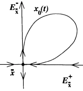
As an example of a system for which there are exponential dichotomies on R+ and ]R but not on R consider the planar autonomous differential equation, : i; =f (x) sketched in figure 2.1.
Figure 2.1: xo(t) is a solution which is homoclinic to the hyperbolic saddle T.
[image:29.582.225.358.474.620.2]dichotomy on R+ and R-. " However, since the (one dimensional) forward and backward contracting manifolds of x coincide along xo, their tangent spaces, E+ (t), c
and Exo(t), t must also coincide. But these are the forward and backward contracting subspaces for the linearisation and so cannot have direct sure R2. Thus there is no
exponential dichotomy on R.
If however we perturb to get x=f (x)+sg(t) then we can look for solutions xE(t) homoclinic to the nearly-fixed point ±E. If x, (t) exists, then generically, it will have an exponential dichotomy and thus correspond to a transversal intersection of the stable and unstable manifolds of xE. It is then known as a transversal hornoelinic solution. The existence of transversal homoclinic solutions allows one to deduce many interesting results. For example, if there are many such intersections then the nearby dynamics can be extremely complex. For a treatment of the case where
g is periodic the reader is referred to Palmer [321, who uses the theory of exponential dichotomy to derive a Melnikov type function for the existence of xE and also to deduce the existence of random dynamics near to xE. This can also be done for aperiodic forcing. Gruendler [13] has some answers in this direction and in principle one could use the theory developed in this thesis to provide an elegant quantitative approach to this problem.
2.3
A useful characterisation
of hyperbolicity
The study of hyperbolicity for solutions of (2.1) or equivalently exponential dichotomy for (2.2) can be reduced to the study of a linear differential operator on suitable function spaces. This is fundamentally the approach I take in order to treat aperiodic systems in an appropriate manner.
It will prove advantageous to think of x=f (x, t) as a differential equation on
C1 functions x: IR -+ R7 rather than on vectors xE iR". By definition, for xE C'
we have
xE C°. It follows from the hypotheses on the vector field f (x, t) that for
xE C1, the right
hand side f (x(t), t), is a bounded CO function. Thus the vector
field can be regarded as the operator f: C1 -f CO, f (x) (t) Hf (x (t), t). Moreover,
since f
(x, t) is uniformly C' with respect to xE Rn, it follows that the operator f
is C1 with respect to functions xE C1 as well.
Define C1, the space of C1-vector fields, by d' = C' (C', C°). This clearly contains
the vector fields we are interested in but in fact it is much larger and contains
operators which are not really vector fields at all. For our purposes however, this is not a problem. In fact, it allows us to show robustness to a much more general class of perturbations, for example, where the time dependence is more complicated
such as differential-delay equations. The norm I will use on d' is
if ýýcl = sup max { HHf(x('), ')Ilc(, , IlDf.,, Ilci-4co }
xEC'This is a generalisation of the norm on C' vector fields used in standard dynamical systems theory. "' Note that Dff(t) = Dfý, (t), t.
Consider the nonlinear operator, G: C1 -+ C°, defined by G(x)(t) = j7 (t) -f (x (t), t)
In this context we have the following reformulation of definition 2.1. Definition 2.10 xE C1 is a bounded solution of (2.1) if G(x) = 0.
The linearisation of G about a solution xo E C', is C= L)GxO
: C' -+ CO, given
by
Gd
dt -Dfo
Note that all the C1 solutions of the variational equation (2.2) are obtained by solving Gý = 0.
2.3.1
Green's
functions
and the inhomogeneous
variational
equation
It is well known that the exponential dichotomy of the variational equation is
closely related
to the solvability of the inhomogeneous equation
ý=D. f,;
oý+ýp
(2.10)
where cp E C°. All the C' solutions of (2.10) are given by solving C=V. To do this we look for a two-point function of time associated with C called a Green's function. As we are interested in obtaining bounded solutions rather than particular initial value problems or boundary value problems I only consider the relevant Green's
function.
Definition 2.11 For the first order linear differential operator L: C' -ý C° defined above, a Green's function an essentially bounded matrix-valued operator, W: 1I x R -* BL(Rn, R''2), such that for each sER, W satisfies
1. LW(t, s) =0 for t0s
2. limt. +s+ W (ti s) - 1imt, s- W (t, s) =I
There is also a more direct way of characterising W. Let Sr be the distribution defined by St[co] = co(t), for suitable R-valued test functions, cp. For some details of the theory of distributions'" see section 4.2. St is the Dirac delta function or unit impulse (at time t).
Proposition 2.2 W is a Green's function for G, if and only if, for each s, W(., s) is an essentially bounded solution of the distributional equation
LW(-,
S) = bs
For this reason the Green's function is also known as the impulse response.
Proof
To see that this is equivalent to Definition 2.11 notice that property 1 is
trivially satisfied and property 2 follows from
I=
8s
[I] = CW(t, 8) [1]
s+h d
l im dW (t, s) - Dfýo(t) W (t, s) dt
f-h
= hill W (t, s) - lim W (t, s) t-)s+ t->s+
When there is a Green's function there is an explicit expression for solutions of
(2.10). This is given by
(c-'
)(t) =fW
(t, s)w (S) (IS
(2.11)
To see (2.11) gives a solution of
(2.10) we can differentiate to give
dt(G
1`P)(t)
=J
dtW
(t's)ýP(s)ds
= Dffo(t)
fW(t,
s)(s)ds + cp(t)
= Df,; o(t)
(G-I ýp)(t) + ýo (t)
(2.12)
i° For now the details of the theory of distributions are unimportant. Basically, distributions are functionals defined by their action on a suitable space of `test' functions (with compact support).
where Xs(t) = Xo(t)Xo 1(s) is the fundamental solution of the homogeneous varia- tional equation satisfying Xe(s) = I.
Fort> s, W(t, s)EEt and fort< s, W(t, s)EEt .
To see that this satisfies definition 2.11 notice that it is bounded and =I tum W (t, s) - tJiym W (t, s) = X0(t)P0Xo 1(t) + Xo(t)(I - P0)Xo '(t)
By construction it satisfies JW (t, s) j< KeaIt-. Sl and thus W (t, ") E L1 with the
uniform bound IIW (t, ") I I1 < 2K/a.
Some more details of this method of solving (2.10) are given in the next chapter where it is a crucial part in providing persistence estimates for hyperbolic solutions. Perron was the first to notice that questions about the homogeneous equation, - A(t)e, were closely related to the solvability of the inhomogeneous equation, - A(t)e +" Massera & Schaffer [26] first developed this line of attack formally. They called the pair of function spaces (A, 8), admissible for C. if L: A -+ B was surjective. One of the basic theorems they proved is that L: Cl(I) -+ C°(Z) is surjective if and only if the variational equation (2.2) has an exponential dichotomy on Z.
For half-lines the theorem is stated as
Theorem 2.4 (2.2) has an exponential dichotomy on 1Rt if and only if C: C j' - C, is surjective.
Proof
[ED =
Surj]
Suppose there is an exponential dichotomy on R+ with projection P. S. Then we
can define a
Green's function on R+ as follows.
stisi0
W (t, s)
-X
Xs(t) P
(2.15)
s
(t) (I
- P3)
0<t<8
A C+ solution of L=
cp for any cp E C+ is then given by
(L-10(t) =JW
(t, s) v (s) ds
[Surf =
ED]
Let Vi be the subspace of IR' which contains all the initial conditions which generate bounded solutions (on R+) of the variational equation. That is,
If for each tER, we have" W(t, ") E LI, and for some Al independent of t, IIW(t,
")Il1 =J IW(t, s)lds <M <C)0 then (2.11) gives a C1 solution of (2.10).
To see this, observe that uniform boundedness of C-' (p follows from Hölders
inequality' which gives
ll,
c-,
(Pll.
koll".
From (2.12) it follows that dt(G-l(p) is bounded if G-lcp is. Clearly,
dt(G
1(P)II <_ (IIDf,,
00
oll IIW(t, )III + 1) IIýIIý
So G-1 is an integral operator with Green's function kernel. If W is the unique,
L1 Green's function then C-1 gives the unique C' solution of (2.10) and satisfies
IJG-'j1cl
< max{IIW(t,.
)III
, IHDf.,,,
IH
IIW(t,.
)Ill + 1}
The Green's function for a hyperbolic solution
Proposition 2.3 When x0 is hyperbolic, there is a unique, L1 Green's function for G. Moreover it satisfies the estimate
W (t, S)I < Ke it-sI
where K, a are the hyperbolicity constants.
Proof
For each s, W(-, s) should be a bounded matrix solution of
C-
Df
0
(, s) = Ss
(2.13)
dt
W
)
By hyperbolicity, for any column ý, of W(-, s) we have
jPtý(t)I >_ Ke'(t-s) Iý(S+)I ýI
- Pt)ý(t)I >_ Kea(s-t) Iý(s )I
Thus for bounded solutions of (2.13) we require Ptý(t) =0 for t<s
and
(I - Pt)ý(t) =0 for t>s. This is enough to see that Wt should be
W(t, S) =
XS(t)P8
t>
.5
(2.14)
-X, (t)(I - P3)
t <s
considered as a the matrix-valued function W (t, .): II8 -3 BL(R? i, R n)
Let V2 be any complementary subspace and let Po be the projection which satisfies Range Po = Vl and ker Po = V2. Then we can define a Green's function W (t,, s) by (2.15) above. This is clearly bounded and satisfies definition 2.11
The proof is completed by showing that when L is surjective, JW (t,, s) l< Ke_ t_8l, from which it follows that Po is the projection on to the forward con- tracting subspace. The details, which are messy, can be found in [9] or [7].
This result is also true for R but we can say a little more. Theorem 2.5 The following are equivalent
" xO is hyperbolic.
"G:
Cl --p CO is surjective.
"
C° is invertible.
[Hyp]
[Surj] [In3 + Surf] Proof
[Hyp = Surj]
If there is an exponential dichotomy on R then by proposition 2.3 there is a unique, L1 Green's function given by (2.14) and thus a unique, C1 solution of Q= cp for any ýp E C°.
[Hyp = Injl
If (2.2) has an exponential dichotomy on R (with projection PO) then it has no non-trivial bounded solutions since the evolution of any initial condition with non-zero component in Po (resp. I- P°) is unbounded in backward (resp. forward)
time. Thus L is injective. [Surj ; Hyp]
Clearly, if L is surjective on CO then it is also surjective on C. ý and CO-. By theorem 2.4, the variational equation (2.2) must have an exponential dichotomy on R+ and R and clearly the projections are the same. By theorem 2.3 we deduce that (2.2) has an exponential dichotomy on R.