Oscillatory flow and temperature fields in an open tube with temperature difference across the ends

warwick.ac.uk/lib-publications

Original citation:

Rajan, A. T. , Narasimham, G. S. V. L. and Jacob, Subhash. (2011) Oscillatory flow and temperature fields in an open tube with temperature difference across the ends. International Journal of Heat and Mass Transfer, 54 (15-16). pp. 3357-3368.

Permanent WRAP URL:

http://wrap.warwick.ac.uk/81412

Copyright and reuse:

The Warwick Research Archive Portal (WRAP) makes this work by researchers of the University of Warwick available open access under the following conditions. Copyright © and all moral rights to the version of the paper presented here belong to the individual author(s) and/or other copyright owners. To the extent reasonable and practicable the material made available in WRAP has been checked for eligibility before being made available.

Copies of full items can be used for personal research or study, educational, or not-for-profit purposes without prior permission or charge. Provided that the authors, title and full

bibliographic details are credited, a hyperlink and/or URL is given for the original metadata page and the content is not changed in any way.

Publisher’s statement:

© 2016. This manuscript version is made available under the CC-BY-NC-ND 4.0 license http://creativecommons.org/licenses/by-nc-nd/4.0/

A note on versions:

The version presented here may differ from the published version or, version of record, if you wish to cite this item you are advised to consult the publisher’s version. Please see the ‘permanent WRAP URL’ above for details on accessing the published version and note that access may require a subscription.

Final version

Oscillatory flow and temperature fields in an open tube with

temperature difference across the ends

T.R. Ashwina_{, G.S.V.L. Narasimham}a,∗_{, Subhash Jacob}b a_{Department of Mechanical Engineering}

b_{Centre for Cryogenic Technology}

Indian Institute of Science, Bangalore 560012, India

Abbreviated title: Oscillating flow in a tube

Abstract: The oscillating flow and temperature field in an open tube subjected to cryogenic

temperature at the cold end and ambient temperature at the hot end is studied numerically.

The flow is driven by a time-wise sinusoidally varying pressure at the cold end. The conjugate

problem takes into account the interaction of oscillatory flow with the heat conduction in the

tube wall. The full set of compressible flow equations with axisymmetry assumption are solved

with a pressure correction algorithm. Parametric studies are conducted with frequencies of

5-15 Hz, with one end maintained at 100 K and other end at 300 K. The flow and temperature

distributions and the cooldown characteristics are obtained. The frequency and pressure

amplitude have negligible effect on the time averaged Nusselt number. Pressure amplitude is

an important factor determining the enthalpy flow through the solid wall. The frequency of

operation has considerable effect on penetration of temperature into the tube. The density

variation has strong influence on property profiles during cooldown. The present study is

expected to be of interest in applications such as pulse tube refrigerators and other cryocoolers,

where oscillatory flows occur in open tubes.

Keywords: Pulsating flow, Pulse tube, Heat transfer, Laminar, Circular tube, Conjugate

convection.

∗:Corresponding author. Telephone: +91-80-22932971, Fax: +91-80-23600648

Nomenclature

cp constant pressure specific heat (J kg−1K−1)

D,d diameter (m)

˙

E enthalpy flow (W)

Ec Eckert number, v2

c/cp,cTc dimensionless

f frequency (Hz)

g acceleration due to gravity (m s−2₎

H length of tube (m)

h heat transfer coefficient (W m−2_K−1₎

k thermal conductivity (W m−1K−1)

L length m

˙

M mass flow rate kg s−1

N u Nusselt number,h Ri/k dimensionless

p pressure (Pa)

P r Prandtl number,µ cp/k dimensionless

R radius (m)

Re Reynolds number,ωR2

i ρ/µ dimensionless

T temperature (K)

t time (s)

Greek Symbols

∆Tc characteristic temperature difference K

γ ratio of specific heats dimensionless

overheat ratio dimensionless

µ dynamic viscosity (kg m−1_s−1₎

ν kinematic viscosity (m2s−1)

ρ density (kg m−3₎

ω angular frequency (rad s−1)

Subscripts

a amplitude

av average

c characteristic

e evaporator or cold

f fluid region

h hot or ambient

i inner

o outer, charge pressure

p time period

r radial direction

s solid region

w wall

z axial direction

Superscript

* dimensionless quantity

1

Introduction

Oscillating flow through passages like pipes and conduits is of interest in biological applications

in relation to blood flow, industrial heat exchangers, manifolds, combustion and regenerators

of Stirling and pulse tube cryocoolers. In the studies aimed at determining the heat transfer

and friction between the wall and oscillating flow, the pulsatile flow field is assumed to consist

of a steady Poiseuille flow part and a purely oscillatory part. Such a flow could enhance

heat transfer by breaking down the boundary layer. In other words, the pulsations can have

considerable effect on the rate of heat transfer and thermal resistance due to the alteration

of thickness of the thermal boundary layer [1]. The flow and temperature distributions that

occur in oscillatory flow in a tube with the end portions of the tube maintained at different

temperatures is of interest in pulse tube refrigerators. The present study is motivated by such

an application. Due to the nature of the problem and the large temperature differences that

exist, the problem is analyzed using the full set of compressible flow governing equations with

the assumption of axis symmetry.

Faghri et al. [2] reported a study on the heat transfer from a cylindrical pipe where

periodic flow is superimposed on a fully developed steady laminar flow. It was shown that the

interaction between velocity and temperature pulsations generates an extra diffusivity akin to

eddy diffusivity, contributing to larger heat transfer rates.

There are other numerical investigations such as those of Cho et al. [3] which focused

at-tention on heat transfer characteristics of a pulsating flow in a pipe. Using unsteady

boundary-layer equations, Cho et al. [3] found that the time-mean axial velocity profiles and the Nusselt

number were largely unaffected by the changes in frequency parameter and amplitude of

os-cillation. The skin friction was found to be greater than that of steady flow. The influence of

Amir et al. [4] presented a correlation for the prediction of the heat transfer coefficient in

a heating process for steady and pulsating flow of air through a circular pipe. The pulsating

frequency is between 5 and 60 Hz and a combined dimensionless number composed of the

Reynolds number and a dimensionless flow frequency was used to correlate thermal behavior

with flow parameters. When this number was below 2.1 × 105_{, there was no significant}

improvement in heat transfer. Similar work was reported by Chattopadhyay et al. [5] for

simultaneously developing pulsating incompressible laminar flow in a pipe with constant wall

temperature. The analysis proved that pulsation has a negligible effect on time-averaged heat

transfer. Moschandreou et al. [6] reported that the rate of heat transfer is not significantly

affected when the frequency is very low or very high, while Guo et al. [7] reported that heat

transfer augmentation occurs at large amplitudes of oscillation. For turbulent pulsating flow,

Wang [8] found that there exists an optimum Womersley number at which heat transfer is

enhanced. Heat transfer characteristics of pulsating turbulent air flow in a pipe heated at

uniform heat flux were experimentally investigated [9]. The results show that the Nusselt

number is strongly affected by pulsation frequency, the relative Nusselt number increasing

or decreasing depending on the frequency range. Zhao et al. [10] presented a heat transfer

correlation in terms of the kinetic Reynolds number, dimensionless amplitude of oscillation,

length-to-diameter ratio and the Prandtl number. Khabakhpasheva et al. [11] experimentally

observed considerable phase shift between the velocity and pressure gradient in pulsating flows

of viscoelastic fluids.

Hemida et al. [12] studied the pulsation effect on heat transfer in laminar incompressible

flow in a duct for both thermally fully developed and developing conditions. The results show

that the pulsation has negligible role in fully developed region but it has greater sensitivity

in thermally developing region. For isothermal and isoflux boundary conditions, the effect

of pulsation on the time average heat transfer coefficient tends to be negative, but remains

relatively small. But non-linear boundary conditions (e.g. radiation and natural convection)

combined with pulsation resulted in a noticeable enhancement of the time average Nusselt

number.

Other studies on pulsating turbulent flows include those of Li and Xu [13], Pascale et al.

[14] and He et al. [15].

From the literature, it can be seen that pulsating gas flow in open tubes subjected to

end-to-end temperature difference and its interaction with the tube wall has not received attention.

Such flows find practical application in various cryocoolers and other thermal systems. In an

earlier paper, the present authors reported a numerical simulation for the complete pulse tube

refrigerator operating high frequencies [16]. The present paper is motivated by the need for a

detailed study of the pulse tube for systems in the frequency range 5-15 Hz.

2

Formulation

2.1

Geometry

Fig. 1 shows the physical model and coordinate system. Cylindrical polar coordinate system

is chosen with the assumption of axisymmetric flow and temperature distributions. The model

consists of a cylindrical pipe with finite wall thickness and both the ends open. The flow and

temperature distributions are assumed to be axisymmetric. Ther-axis is perpendicular to the

vertical axis and points outwards in a radial direction. The positive direction of the z-axis

coincides with the vertical axis and points upwards. The gravity vector is parallel to thez-axis

and acts vertically downwards. The portions of the tube beyond the open ends belong to the

entering one of the ends does so at a cryogenic temperatureTe. Similarly the working medium

entering the other end of the tube is at a higher temperature Th. The oscillating flow in the

tube is driven by a sinusoidally varying pressure at the cold end of the tube. Since the so

called DC component is absent, the fluid flow during a cycle takes place partly into and partly

out of the tube at either end. The height of the tube and the inner and outer radii are H,Ri

and Ro, respectively. Clearly the wall thickness δw is Ro−Ri. The oscillating heat transfer

between the wall and the gas is taken into account through the coupling between the fluid

and the solid at the interface. The annular surfaces of the solid at the tube ends are assumed

to be insulated.

2.2

Non-dimensionalisation

The characteristic length Lc is taken as the inner radiusRi of the tube and the characteristic

temperature Tc as the hot heat exchanger temperatureTh, which is the ambient temperature.

The geometrical parameters of the problem are the dimensionless inner radius R∗_i of the tube,

dimensionless height H∗ and the dimensionless wall thickness δ_w∗. The characteristic density

ρc corresponds to the state of helium at the charge pressure po and ambient temperature

Th = Tc. The characteristic thermal conductivity, specific heat and dynamic viscosity of the

working medium, i.e. helium gas, correspond to Tc and are denoted respectively kc, cp,c and

µc. The dimensionless temperature T∗ is (T −Tc)/∆Tc where ∆Tc is Th−Te. The quantity

= ∆Tc/Tc is the overheat ratio. The characteristic pressure is pc is taken asρcvc2 where vc,

the characteristic velocity, is taken as ωLc. The time is non-dimensionalised with the time

period of the oscillation 1/ω. Thus the dimensionless time period t∗_p is 2π.

The dimensionless quantities are defined as:

t∗ =tω, r∗ = r Lc

, z∗ = z Lc

, Lc =Ri

v∗_r = vr vc

, v∗_z = vz vc

, p∗ = p ρcv2c

, vc =ωLc

T∗ = T −Tc ∆Tc

, = ∆Tc Tc

, ∆Tc=Th−Te, Tc =Th

ρ∗ = ρ ρc

, c∗_p = cp cp,c

, µ∗ = µ µc

, k∗ = k kc

Re= vcLcρc µc

, P r= µccp,c kc

, Ec = v 2 c cp,cTc

H∗ = H Lc

, δ_w∗ = δw Lc

The dimensionless outer radius is R∗_o = Ro/Lc = 1 + δw∗ and the dimensionless charge

pressure p∗_o =po/(ρcv2c). The dimensionless properties should correspond to the fluid or solid

depending upon the region under consideration, i.e. the working medium or wall. Thus the

dimensionless ratios, namely, µ∗_f, c∗_p,f and k_f∗, the subscript ’f’ denoting fluid, are assigned a

value of unity in the fluid domain. In the solid region, the property values should correspond

to those of the solid, namely,k_s∗andc∗_s =cs/cp,c. In the numerical analysis, the solid is treated

as a fluid of infinite viscosity.

2.3

Dimensionless governing equations

The dimensionless continuity, momentum and energy equations are as follows:

Continuity equation

∂ρ∗ ∂t∗ +

1 r∗

∂ ∂r∗(r

∗

ρ∗v_r∗) + ∂ ∂z∗(ρ

∗

v∗_z) = 0 (1)

∂ ∂t∗(ρ

∗

v∗_r) + 1 r∗

∂ ∂r∗(r

∗

ρ∗v_r∗v∗_r) + ∂ ∂z(ρ

∗

v_z∗v_r∗) =−∂p

∗

∂r∗ +

1 Re 1 r∗ ∂ ∂r∗

r∗µ∗∂v

∗ r ∂r∗ + ∂ ∂z∗ µ∗

∂v∗_r ∂z∗

+Sr (2)

Momentum equation in axial direction

∂ ∂t∗(ρ

∗

v∗_z) + 1 r∗

∂ ∂r∗(r

∗

ρ∗v_r∗v∗_z) + ∂ ∂z∗(r

∗

ρ∗v∗_zv_z∗) =−∂p

∗

∂z∗ +

1 Re 1 r∗ ∂ ∂r∗

r∗µ∗∂v

∗ z ∂r∗ + ∂ ∂z∗

µ∗∂v

∗ z ∂z∗

+Sz (3)

Energy equation

∂ ∂t∗(ρ

∗

T∗) + 1 r∗

∂ ∂r∗(ρ

∗

r∗v_r∗T∗) + ∂ ∂z∗(ρ

∗

v_z∗T∗) = 1 ReP r 1 r∗ ∂ ∂r∗ k∗ c∗ p

r∗∂T

∗ ∂r∗ + ∂ ∂z∗ k∗ c∗ p ∂T∗ ∂z∗ + Ec c∗ p Dp∗

Dt∗ (4)

Equation of state

p∗ = 1 Ecρ

∗ γ−1

γ (T

∗

+ 1) (5)

The momentum source terms are given by:

Sr = 1 Re ∂ ∂z∗

µ∗∂v

∗ z ∂r∗ + 1 r∗ ∂ ∂r∗

r∗µ∗∂v

∗ r ∂r∗

−2µ

∗_v∗ r r∗2 −

2 3

∂ ∂r∗(µ

∗

D∗)

(6)

Sz= 1 Re ∂ ∂z∗ µ∗

∂v_z∗ ∂z∗ + 1 r∗ ∂ ∂r∗

r∗µ∗∂v

∗ r ∂z∗ − 2 3 ∂ ∂r∗(µ

∗

D∗)

(7)

where the dimensionless divergence is given by:

D∗ = 1 r∗

∂ ∂r∗(r

∗_v∗ r) +

∂v_z∗ ∂z∗

The substantive derivative Dp∗/Dt∗ is given by:

Dp∗ Dt∗ =

∂p∗ ∂t∗ +v

∗ r

∂p∗ ∂r∗ +v

∗ z

∂p∗ ∂z∗

2.4

Nusselt number and enthalpy flow

The Nusselt number at any axial location on the fluid-solid interface and at any time is defined

as

N uz=

∂T∗ ∂r∗

r∗_=R∗ i

(8)

The Nusselt number N uav is the average of N uz over the length of the interface and one

time period.

N uav = 1 H∗_t∗

p

Z H∗

0

Z t∗p

0

N uzdz dt (9)

The enthalpy flow through any cross-section is calculated as:

˙ Eav =

1 π R∗2

i

Z R∗_i

0

ρ∗v_z∗c∗_pT∗(2π r∗dr∗) (10)

2.5

Initial and boundary conditions

It is assumed that at the beginning (i.e. t∗ = 0), the geometry is under ambient condition

and the system is filled with helium gas at the charge pressure. These conditions are taken as

300 K and 25 bar.

No-slip and zero mass permeability is assumed on the solid boundary in contact with the

fluid. Oscillating pressure and zero radial velocity are prescribed at the cold end of the tube.

At the hot end of the tube, zero streamwise derivative of the radial velocity is prescribed. The

axial velocities at the inlet and outlet are calculated using the continuity equation. On the

axis of the tube, zero cross-stream derivative of the axial velocity and zero radial velocity are

At the interface between the solid and the fluid, heat flux continuity and no temperature

jump conditions should be satisfied. This is done through the harmonic mean thermal

con-ductivity method [18]. At the cold end, the temperature condition is taken as the cold heat

exchanger temperature when the flow takes place into the tube and as zero axial temperature

gradient when the flow is out of the tube. Similar conditions are also applied at the hot end

of the tube.

The initial and boundary conditions can be expressed as follows in dimensionless form:

At t∗ ≤ 0: v∗_r = v_z∗ = 0, T∗ = 1 and p∗ = pc/(ρcv2c) (throughout the computational

domain). The quantity vc is given by ωLc.

v∗_r(0, z∗, t∗) = 0; v∗_r(1, z∗, t∗) = 0; v∗_r(r∗,0, t∗) = 0;

∂v∗_r ∂z∗(r

∗

, H∗, t∗) = 0; ∂v

∗ z ∂r (0, z

∗

, t∗) = 0 (11)

The last relation states that the radial derivative of axial velocity is zero on the axis in

view of the symmetry.

The boundary conditions for the temperature at the open ends can be expressed as follows:

If v_z∗(r∗,0, t∗)≤0 then ∂T

∗

∂z∗(r ∗

,0, t∗) = 0

If v_z∗(r∗,0, t∗)>0 then T∗(r∗,0, t∗) = −1.0

If v_z∗(r∗, H∗, t∗)>0 then ∂T

∗

∂z∗(r ∗

, H∗, t∗) = 0

If v_z∗(r∗, H∗, t∗)≤0 then T∗(r∗, H∗, t∗) = 1.0 (12)

At the interface:

−k_f∗∂T

∗ f

∂r∗ =−k ∗ s

∂T_s∗ ∂r∗; T

∗ f =T

∗

s (13)

The pressure oscillation at the inlet of the pipe is:

p∗(t∗) = p∗_o+p∗_asin(t∗) (14)

where p∗_o is the dimensionless charge pressure.

3

Numerical method

The governing equations are discretized on staggered mesh. Fig. 2 shows the nodalized

rep-resentation of the quantities on a staggered mesh [17]. The pressure, density, temperature

and gas properties are defined at the control volume nodes. The radial and axial velocities

are defined at the faces of the control volumes, as shown. Velocities required elsewhere are

obtained by linear interpolation with respect to the grid metrics. The algebraic

transfor-mation of Roberts [22] is used in the radial direction for obtaining finer mesh at the axis

and the solid-fluid interface. The solution is obtained by the SIMPLEC algorithm of Van

Doormal and Raithby [19]. The time derivatives are approximated by backward differences

and the diffusive terms, by central differences. For convective terms, the third-order accurate

HLPA (Hybrid Linear and Parabolic Approximation) scheme is Zhu [20] is employed due to

its good transportive property, upwind bias and lower false diffusion. The discretized

equa-tions in five point stencil form are solved using the Modified Strongly Implicit Procedure of

Schneider and Zedan [21]. This solver, though iterative in nature, achieves a high degree of

implicitness, characteristic of direct methods. The time step depends on the frequency and

pressure amplitude. Typically each time period is divided into 400-800 time steps. The solid

region is considered as a fluid region with infinite viscosity and appropriate density, specific

heat and thermal conductivity. Following startup, the system reaches a periodic state after

a sufficient time has elapsed. The time marching is continued until periodic conditions are

achieved. Sufficient number of global iterations are performed at each time step. During each

global iteration, the velocities, pressure correction, temperature and density are determined

the residuals for continuity and energy are better than 10−3.

Grid dependency of the results is checked by varying the grid size in the axial and radial

directions. The axial divisions are varied from 100 to 200 and the radial divisions in the fluid

from 10-15, with three nodes deployed in the wall region. The area-average velocity is plotted

for two cases at the middle cross-section in Fig. 3. The mesh with 100 axial divisions is found

to perform almost similar to that with 200 divisions. Grid sensitivity tests are also conducted

for various Reynolds numbers and the 15×100 grid is found to be adequate for the geometry

selected.

4

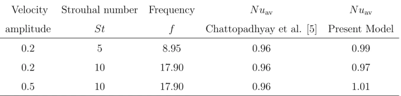
Validation of the computer code

The present code is validated against the simulation of Chattopadhyay et al. [5]. For this

purpose, the present code was modified to incorporate oscillating velocity and isothermal wall

boundary conditions. The validation is conducted for a Reynolds number of 200, for various

velocity amplitudes and for frequencies below 20 Hz. A mesh with 100 control volumes in

the radial direction and 800 control volumes in the axial direction was chosen. The frequency

is adjusted to match the Strouhal number chosen in the original work. The results of the

validation study presented in Table 1 show a favourable agreement between the two studies.

5

Results and discussion

5.1

The effect of pressure amplitude

Figures 4 and 5 show the temperature and velocity distributions inside the tube for pressure

amplitude of 50 Pa and 500 Pa after 66 seconds. At this time the flow reversal is about to take

K, the initialization temperature being 300 K. This shows that the temperature at the cold

end stars penetrating into the tube and a temperature gradient is being setup in the tube.

With open ends, it can be observed that a small pressure oscillation at the inlet results in large

axial velocity gradient. The pressure amplitudes are kept low in order to prevent smearing of

the temperature profiles by the large axial velocities in the tube. Because of the onset of the

flow reversal at this time the velocities in the tube are very small. The flow reversal is mostly

confined to the central part of the tube. The flow pattern suggests that there is a possibility

for the occurrence of eddy formation at the entrance and exit in the central part of the tube.

The axial variation of wall temperature for two pressure amplitudes is presented in Fig.

6 for the middle cross-section of the tube wall at the mid thickness after 167 seconds for a

frequency of 15 Hz after attaining periodic conditions. The attainment of periodic conditions

is ensured by plotting the temperature distribution for two successive time periods and by

observing that there is no change in these profiles. The mid thickness wall temperature at the

tube inlet for the two the cases are different. For the first case with 50 Pa pressure amplitude,

the solid cold end temperature is 183.38 K where as in the second case, the same is 142.37

K at the cold end. The wall to gas temperature difference in these two cases are respectively

83.38 K and 42.37 K. The reason is traced to the fact that higher pressure amplitudes result in

higher velocities and lower thermal boundary layer thickness. It is observed, however that that

the hot end temperature of the tube wall does not change much with pressure amplitudes, the

wall to gas temperature difference at the hot end being very small, typically, 10 K for the first

case and 15 K for the second case. Thus higher pressure amplitude appears to be lowering the

cold end temperature of the wall and maintaining more or less the same hot end temperature.

This can also be verified from the Table 2 which shows higher energy flow through the solid

density of the fluid at the cold end and lower density at the hot end. Moving away from the

cold end to the hot end, the disturbances decrease and the rate of temperature change also

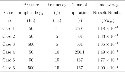
decreases (Fig. 6). From Table 3, it can also be seen that the values of the average Nusselt

number are rather lower compared to incompressible flow [5] and do not change much with

frequency of operation or pressure amplitude. It should be noted that both ends and outer

surface of the tube are insulated and therefore there the only thermal interaction between the

gas and solid is through the interface. This observation is analogous to that of Himadri et

al. [5] for incompressible flow. It may be recalled here that the Nusselt number is based on

the difference between the hot and cold end temperatures rather than the difference of the

time-averaged interface and bulk fluid temperatures.

Fig. 7 shows the variation of space averaged Nusselt number and variation of velocity over

one cycle after 167 seconds of operation from startup. The pressure amplitude is 50 Pa and

the frequency is 15 Hz. The variation in the Nusslet number over a cycle is found to stabilize

after attaining periodic condition. The value of Nusselt number increases and decreases during

a cycle. The variation of the cross-section averaged velocity is also shown in this Figure. The

variation in the Nusselt number follows the same pattern as that of the average velocity over

one cycle.

The radial velocity corresponding to an instant is plotted against the axial velocity at the

same instant in Fig. 8. The location of the monitoring point is at the mid radius and at the

mid length of the tube, the frequency and amplitude being 15 Hz and 50 Pa. Since the curve

closes on itself, it can be concluded that the cooldown phase is passed and the flow field has

become fully periodic.

Fig. 9 shows the area-averaged axial velocity profiles after 6.66 seconds and 167 seconds

of operation at the middle cross section of the tube. The observations are taken for a case

of 500 Pa amplitude and 15 Hz frequency. Though the shorter time and longer time profiles

are similar in shape, the profile is found to shift downwards as the periodic state approaches.

Although not shown here, such a marked shift is not observed between the shorter time and

longer time temperature profiles. This can be due to the strong influence of density variation

in the beginning of the operation. All the cases are initialized with ambient condition at the

startup. The thermal effect of the cold end diffuses into the tube and causes a strong density

variation influencing thereby the velocity profiles inside the tube. This kind of distortion has

earlier been reported by the authors in a previous study on a pulse tube refrigerator at higher

frequencies [16].

Fig. 10 shows the cooldown characteristics for 15 Hz frequency and 500 Pa pressure

amplitude at the middle of the tube. The non dimensional temperature plotted is the area

average over the cross-section. Time advancement is executed until the temperature variation

of two consecutive cycle stabilizes. The best fit for the cooldown characteristic data in terms

of dimensionless temperature and dimensionaless time, is given by:

T∗ = −8.08×10−3−9.11×10−5t∗+ 3.14×10−8t∗2−6.32×10−12t∗3

+6.52×10−16t∗4−3.27×10−20t∗5+ 6.35×10−25t∗6 (15)

The average absolute deviation for the above fit is 0.0072 and the multiple correlation is

0.976. The above equation is valid for the dimensionless time ranges presented in Fig. 10.

5.1.1 Effect of frequency

Fig. 11 shows the variation of temperature at the middle cross section of the tube over one

cycle for frequencies of 10 Hz and 15 Hz. The different temperature scales for the lower and

the frequency increases, the temperature penetration into the tube becomes deeper. The inlet

temperature could cool the gas in the middle section up to an average value of 269 K with

a temperature amplitude of 0.4 K. For frequency of 10 Hz the cross section temperature is

average 295 K with a temperature amplitude of 0.8 K. From this, it can be observed that the

temperature penetration increases with increase in frequency. For a pulse tube refrigerator,

three fluid zones can be identified; a zone near the cold end, a central zone and a zone near

the hot end. The mixing of gases of cold and hot zone will destroy the cooling effect. Higher

frequency pulse tubes are likely to exhibit mixing of gases between the two end zones because

of deeper temperature penetration. Thus the length to diameter ratio should be properly

adjusted to prevent mixing of gases. The frequency of operation is also an important factor

other than length to diameter ratio, in designing the pulse tube refrigerator [16].

Fig. 12 shows the temperature distribution of gas and solid for a particular instant. The

observations are taken for a model working with frequency 10 Hz and 50 Pa amplitude. The

figure shows a large temperature difference, amounting to 151 K, at the inlet of the tube.

Proper meshing is important in this region to capture the large temperature gradient. The

temperature differences decrease to a value of 10−3 at the exit. The energy transfer between

the wall and the gas decreases with axial distance. The temperature difference at the cold end

is the main source of pumping energy to the wall of the tube. Fig. 13 shows the heat transfer

between the working gas and the wall at middle cross section of the tube after cooldown. The

results indicate that the gas-wall heat transfer is higher for higher frequency systems. Detailed

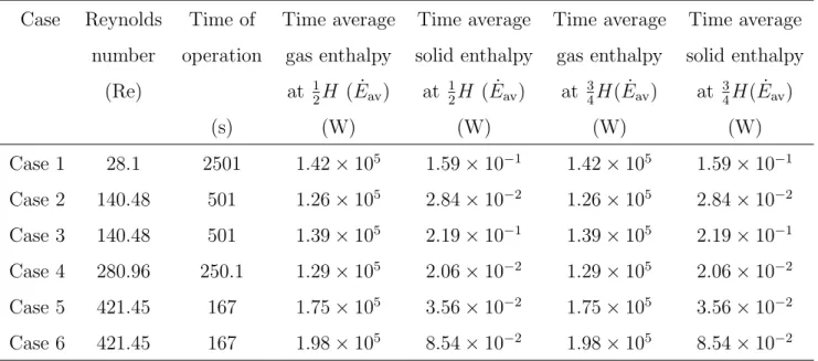
energy balance sheet is given in Table 2. The gas and solid enthalpy flow is calculated at the

middle cross section (i.e. atH/2) and near the exit (4H/3) of the tube. The table shows that

the heat transfer through the solid wall is negligible compared to the enthalpy flow through

the gas. The difference in the cycle average enthalpy flow between the two cross sections is

found to be negligible.

5.2

Phase relationships

Fig. 14 shows the phase relationship between the temperature and mass flow rate at the middle

cross-section of the tube after periodic condition is achieved for frequencies of 10 and 15 Hz.

These are the area-averaged quantities over the cross-section. Such data is very important

for designing devices like pulse tube refrigerator, since the heat released or absorbed directly

depends on the phase relationship between the mass flow and the temperature. Assuming

ideal gas relation, the enthalpy flow over a cycle can be written as:

˙ E = 1

tp

I tp

0 ˙

M cpdt (16)

It can be seen from Fig. 14 that temperature leads the mass flow rate for both the

frequencies. The phase relationship between these quantities depends upon several factors

like geometrical dimensions of the tube, the frequency and the pressure amplitude. Ideally

the temperature should be in phase with the mass flow rate for maximum enthalpy flow rate.

5.3

Conclusions

The problem of oscillating flow inside an open tube with finite wall thickness, ambient to

cryogenic temperature difference at the ends, driven by sinusoidal pressure variation at the

cold end is studied numerically by solving the full set of compressible conservation equations

with axisymmetry. Parametric studies are conducted with different pressure amplitudes and

frequencies. The wall to gas temperature difference is maximum at the cold end and lowest

at the hot end. As the pressure amplitude increases, the temperature difference between the

hot end is less sensitive to the pressure amplitude. The frequency of operation is an important

factor in determining the temperature penetration into the tube. This should be taken into

account for designing devices like pulse tube refrigerators. There is a strong influence of

temperature during cooldown which directly affects the property variations inside the tube.

The pressure amplitude and the frequency have a negligible effect on the time averaged Nusselt

number for the boundary conditions and geometry considered. The result is analogous to the

previous findings for incompressible oscillatory flow. Data on the phase relationship between

the temperature and mass flow rate is useful in designing devices like pulse tube refrigerators.

References

[1] E.G. Richardson, The transverse velocity gradient near the mouths of pipes in which

an alternating or continuous flow of air is established, Proceedings of the Royal Society

London, A42 (1929) 1-15.

[2] M. Faghri, K. Javdani, A. Faghri, Heat transfer with laminar pulsating flow in a pipe,

Letters in Heat and Mass transfer 6 (1979) 259-270.

[3] H.W. Cho, J.M. Hyun, Numerical solutions of pulsating flow and heat transfer

charac-terestics in a pipe, International Journal of Heat and Fluid Flow 11 (1990) 321-330.

[4] A.A. Al-Haddad, N. Al-Binally, Prediction of heat transfer coefficient in pulsating flow,

International Journal of Heat and Fluid Flow 10 (1989) 131-133.

[5] H. Chattopadhyay, F. Durst, S. Ray, Analysis of heat transfer in simultaneously

devel-oping pulsating laminar flow in a pipe with constant wall temperature, International

Communications in Heat and Mass Transfer 33 (2006) 475-481.

[6] T. Moschandreou, M. Zamir,Heat transfer in a tube with pulsating flow and constant

heat flux, International Journal of Heat Mass Transfer, 40 (1997) 2461-2466.

[7] Z. Guo, H.J. Sung, Analysis of the Nusselt number in pulsating pipe flow, International

Journal of Heat and Mass Transfer 40 (1997) 2486-2489.

[8] X. Wang, N. Zhang, Numerical analysis of heat transfer in pulsating turbulent flow in a

[9] A.M.E. Elshafei, M.S. Mohamed, H. Mansour, M. Sakr, Experimental study of heat

transfer in pulsating turbulent flow in a pipe, International Journal of Heat and Fluid

Flow 29 (2008) 1029-1038.

[10] T. Zhao, P. Cheng, A numerical solution of laminar forced convection in a heated pipe

subjected to a reciprocating flow, International Journal of Heat and Mass Transfer 38

(1995) 3011-3022.

[11] E.M. Khabakhpasheva, V.I. Popov, A.N. Kekalov, E.S. Mikhailova, Pulsating flow of

viscoelsatic fluids in tubes, Journal of Non-Newtonian Fluid Mechanics 33 (1989)

289-304

[12] H.N. Hemida, M.N. Sabry, A. Abdel-Rahim, H.Mansour, Theoretical analysis of heat

transfer in laminar pulsating flow, International Journal of Heat and Mass Transfer 45

(2002) 1767-1780.

[13] Z.C. Li, L. Xu, Experimental investigation on the performances of gas flow in

oscillat-ing tube, Proceedoscillat-ings of the Twentieth International Cryogenic Engineeroscillat-ing Conference,

Beijing, China (2004) 257-260.

[14] P. Bouvier, P. Stouffs, J.-P. Bardon, Experimental study of heat transfer in oscillating

flow, International Journal of Heat and Mass Transfer 48 (2005) 2473-2482.

[15] S. He, J.D. Jackson, An experimental study of pulsating turbulent flow in a pipe,

Euro-pean Journal of Mechanics B/Fluids 28 (2009) 309-320.

[16] T.R. Ashwin, G.S.V.L. Narasimham, S. Jacob, CFD analysis of high frequency

minia-ture pulse tube refrigerators for space applications with thermal non-equilibrium model,

[17] F.H. Harlow, J.E. Welch, Numerical calculation of time-dependent viscous incompressible

flow of fluid with free surface, The Physics of Fluids 8 (1965) 2182-2189.

[18] S.V. Patankar, Numerical heat transfer and fluid flow, Series in Computational Methods

in Mechanics and Thermal Sciences, Hemisphere Publishing Corporation (1980)

Wash-ington.

[19] J.P. Van Doormaal, G.D. Raithby, Enhancements of the SIMPLE method for predicting

incompressible fluid flows, Numerical Heat Transfer 7 (1984) 147-163.

[20] J. Zhu, A low-diffusive and oscillation-free convection scheme, Communications in

Ap-plied Numerical Methods 7 (1991) 225-232.

[21] G.E. Schneider, M. Zedan, A modified strongly implicit procedure for the numerical

solution of field problems, Numerical Heat Transfer 4 (1981) 1-19.

[22] G.O. Roberts, Computational meshes for boundary layer problems, Proceedings of the

Second International Conference on Numerical Methods in Fluid Dynamics,

Figure Captions

Fig.1 Physical model and coordinate system.

Fig.2 Location of variables in a staggered mesh.

Fig.3 Results of the grid sensitivity analysis.

Fig.4Temperature and velocity profiles for 15 Hz frequency andpa=50Pa after 66.66 seconds

from startup.

Fig.5Temperature and velocity profiles for 15 Hz frequency andpa=500Pa after 66.66 seconds

from startup.

Fig.6 Wall temperature distribution at two pressure amplitudes.

Fig.7 Variation of the area-averaged velocity at the mid-cross section and that of the wall

Nusselt number over one cycle.

Fig.8 Plot of radial versus axial velocity at mid cross-section and mid radius over a cycle.

Fig.9 Time variation of area-averaged axial velocity at mid cross-section before and after

stabilization.

Fig.10Cooldown characteristics for a frequency of 15 Hz and a pressure amplitude of 500 Pa.

Fig.11 Time variation of area-averaged temperature for frequencies of 10 Hz and 15 Hz.

Fig.12 Axial temperature distribution of gas adjacent to the interface and that of the wall at

mid thickness.

Fig.13 Time variation of the heat transfer between the gas and wall.

Fig.14 Phase relationship between the temperature and the mass flow rate at the middle of

the tube. (a)Frequency 10Hz (b)Frequency 15Hz

List of Tables

Table 1: Results of the validation study

Velocity Strouhal number Frequency N uav N uav

amplitude St f Chattopadhyay et al. [5] Present Model

0.2 5 8.95 0.96 0.99

0.2 10 17.90 0.96 0.97

Table 2: Energy balance for different cases

Case Reynolds Time of Time average Time average Time average Time average

number operation gas enthalpy solid enthalpy gas enthalpy solid enthalpy

(Re) at 1₂H ( ˙Eav) at 1₂H ( ˙Eav) at 3₄H( ˙Eav) at 3₄H( ˙Eav)

(s) (W) (W) (W) (W)

Case 1 28.1 2501 1.42×105 _1.59×10−1 _1.42×105 _1.59×10−1

Case 2 140.48 501 1.26×105 2.84×10−2 1.26×105 2.84×10−2

Case 3 140.48 501 1.39×105 _2.19×10−1 _1.39×105 _2.19×10−1

Case 4 280.96 250.1 1.29×105 2.06×10−2 1.29×105 2.06×10−2

Case 5 421.45 167 1.75×105 _3.56×10−2 _1.75×105 _3.56×10−2

Case 6 421.45 167 1.98×105 8.54×10−2 1.98×105 8.54×10−2

Table 3: Results of the parametric studies

Pressure Frequency Time of Time average

Case amplitude pa (f) operation Nusselt Number

no (Pa) (Hz) (s) (N uav)

Case 1 50 1 2501 1.18×10−1

Case 2 50 5 501 1.33×10−1

Case 3 500 5 501 1.35×10−1

Case 4 50 10 250.1 1.49×10−1

Case 5 50 15 167 1.77×10−1

Figures

Figure 1:

Figure 3:

(a)

(b)

(a)

(b)

Figure 5:

Figure 7:

Figure 9:

Figure 11:

Figure 13:

(a)